Scatterers - Diffuse Polynomial

Navigation: Scatterers > Scatter Types > Diffuse Polynomial

Diffuse Polynomial

Page Contents

Description

Navigation

Controls

Application Notes

•Scatter in transmission and reflection

•Multiple scatter models

•Reading data from a text file

Related Topics

Description

The Polynomial model was developed by Alan W. Greynolds (1994). Most often, a binomial or polynomial scatter model is generated by using the Polynomial Fitting Utility to fit measured data or by bringing in another definition of the same function from another program.

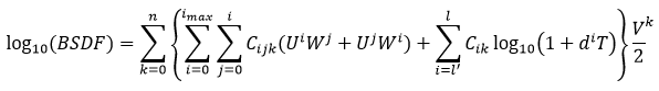
The value of i_maxis the following:

Value of i_max	Condition
m	m > 0
\|m\| - k	(m < 0) and (\|m\| > k)
0	All other cases

In all cases, i_max is always non-negative and the summation i = 0 to i_maxalways has at least one value (i=0) where the summation occurs.

The parameters U, V, W and T have the following meaning, where (a₀,b₀) is the specular direction and (a,b) is the scatter direction.

U = a² + b²

V = aa₀ + b₀

W = a₀² + b₀²

T = (a-a₀)² + (b-b₀)² = U - 2V + W

Navigation

This feature can be accessed by selecting Diffuse polynomia as the Scatter Type in the Create a new scatter model dialog box.

Controls

Control	Inputs / Description	Defaults
Name	Name of the model (required).	Scatter n
Description	Description of the model (optional).
Type	Select Diffuse Polynomial from the pull down menu.	Lambertian
Additional data
n	maximum k counter (n>=0)	0
m	diffuse component counter (m any positive or negative integer)	0
l	maximum j counter (Lorentzian component)	0
l'	minimum j counter (Lorentzian component)	0
d	Lorentzian coefficient (log[specular peak])	0
numA	Number of TIS integration samples in the A direction	201
numB	Number of TIS integration samples in the B direction	201
0	Polynomial coefficients. C(0,0,0) is the lowest order term (constant). The number of coefficients C(i,j,k) increases with increasing n, m & l values.	0
Additional Data
Apply on Reflection	Apply the scatter model on reflection.	Checked
Apply on Transmission	Apply the scatter model on transmission.	Unchecked
Halt Incident Ray	For any surface with this scatter model assigned to it, no specular rays will leave the surface, regardless of the surface coating and raytrace property settings, if this toggle is checked.	Checked

OK	Accept settings and close dialog box.
Cancel	Discard settings and close dialog box.
Help	Access this Help page.

Application Notes

Scattered in transmission and reflection

All scatter models describe the BSDF as measured over a maximum of 2p steradians. Both transmitted and reflected scatter can be modeled by specifying the two scatter directions simultaneously with the appropriate direction controls found under the Scatter tab in the Surface Dialog.

Multiple scatter models

Multiple scatter models can be attached to the same surface. The scatter direction controls are then imposed on every attached model.

Reading data from a text file

Text file data can be read into the Polynomial model by right mouse clicking in the coefficients column and selecting Replace With Data From a File.