|
Description
The Surface Particle (Mie) Scatter model is used to calculate scatter from particulate contamination on otherwise smooth optical surfaces, where the particulates are assumed to be spheres of varying size distributed uniformly on the surface. The size distribution of the particles can take one of several forms: Uniform, Gaussian, mil standard (MIL-1246C or IEST-STD-1246D) or Sampled. The user inputs include the incident wavelength, the real and imaginary parts of the particle refractive index, the minimum and maximum particle diameters, and the particle density. The calculation relies on a numeric integration of the scatter distribution over the range of particle sizes. Calculation of the BSDF proceeds in the following way:
1. The particulate distribution range is divided into N bins (where N depends on the model selected)
2. For each bin:
a) The average particulate diameter is calculated
b) The Mie phase function (intensity) for a single particle per unit area for a given complex refractive index and wavelength is calculated
c) The intensity function is multiplied by the number of particulates in that bin
3. The intensity for all bins is accumulated in summation
4. The BSDF is calculated as
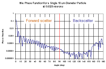
For computational efficiency during the raytrace, the polar angle sampling of the Mie phase function (step 2 above), which is rotationally symmetric, is discretely sampled every 0.1 degrees from 0 to 180 degrees polar angle. As a consequence, the user may notice that the 2D |B-B0| logarithmic scatter plot shows a stepped behavior due to the discretization of the angle binning in the phase function.
.png)
Navigation
This feature can be accessed by selecting Surface Particle (Mie) Scatter as the Scatter Type in the Create a new scatter model dialog box.
Controls
The Surface Particle (Mie) Scatter dialog has the following particulate distribution functional forms: Uniform, Gaussian, MIL-standard. and Sampled.
|
Control
|
Inputs / Description
|
Defaults
|
|
Name
|
Name of the model (required)
|
Scatter n
|
|
Description
|
Description of the model (optional).
|
|
|
Type
|
Choose Surface Particle (Mie) Scatter from the pull down menu.
|
Lambertian
|
|
Model Specification Common Controls
|
|
Wavelen
|
Wavelength in microns for which the scatter model is pre-calculated.
|
Default system wavelength.
|
|
Ref Index
|
Real part of the refractive index of the particles.
|
1.5
|
|
Imag Index
|
Imaginary part of the refractive index of the particles.
|
0
|
|
The following table lists reasonable particulate complex refractive index values at several wavelengths.
|
|
Particulate Complex Index
|
|
Wavelength (microns)
|
Real
|
Imaginary
|
|
0.2
|
1.53
|
0.05
|
|
0.3
|
1.53
|
0.01
|
|
0.4
|
1.53
|
0.005
|
|
0.6328
|
1.53
|
0.0005
|
|
1.15
|
1.5
|
0.001
|
|
3.39
|
1.5
|
0.02
|
|
10.6
|
1.7
|
0.2
|
|
20
|
1.9
|
1.0
|
Reference: Jennings, S., Pinnick, R., Aubermann, H., "Effects of particulate complex refractive index and particle size distribution variations on atmospheric extinction and absorption for visible through middle IR wavelengths", Applied Optics, Vol. 17, pp. 3922-3929 (1978).
|
|
Immerse Index
|
Refractive index of material in which particles are immersed (usually air).
|
1
|
|
Surf Refl
|
Reflectance of surface to which particles are attached. If the model is in reflection, then the forward component of the distribution is multiplied by Surf Refl.
|
1
|
|
Surf Tran
|
Transmittance of surface to which particles are attached. If the model is in transmission, then the forward component of the distribution is multiplied by Surf Trans.
|
1
|
|
(See below for individual particle distribution function controls)
Options are:
MIL-1246C
Uniform
Gaussian
Sampled
IEST-STD-1246D
|
|
Additional data
|
|
Apply on Reflection
|
Apply the scatter model on reflection.
|
Checked
|
|
Apply on Transmission
|
Apply the scatter model on transmission.
|
Unchecked
|
|
Halt Incident Ray
|
For any surface with this scatter model assigned to it, no specular rays will leave the surface, regardless of the surface coating and raytrace property settings, if this toggle is checked.
|
Checked
|
|
|
|
OK
|
Accept settings and close dialog box.
|
|
|
Cancel
|
Discard settings and close dialog box.
|
|
|
Help
|
Access this Help page.
|
|
Uniform Particle Size Distribution
|
Control
|
Inputs / Description
|
Defaults
|
|
The scatter distribution for the Uniform particulate distribution function is constant in direction cosine space. In this distribution the bin count N=31.
|
|
Uniform Distribution Specification
|
|
Density Func
|
Particle size distribution function. Select Uniform.
|
Uniform
|
|
Max. Dia
|
Maximum particle diameter in microns
|
400
|
|
Min. Dia
|
Minimum particle diameter in microns.
|
1
|
|
Density
|
Particle density in particles per square micron.
|
0.1
|
Gaussian Particle Size Distribution
|
Control
|
Inputs / Description
|
Defaults
|
|
The Gaussian particulate distribution gives a strong forward scatter component in the specular direction with a smaller component in the reverse direction. In this distribution the bin count N=29.
|
|
Gaussian Distribution Specification
|
|
Density Func
|
Particle size distribution function. Select Gaussian.
|
Uniform
|
|
Max. Dia
|
Maximum particle diameter in microns.
|
400
|
|
Min. Dia
|
Minimum particle diameter in microns.
|
1
|
|
Density
|
Particle density in particles per square micron.
|
0.1
|
|
Mean
|
Mean particle diameter in microns.
|
10
|
|
Standard Deviation
|
Standard deviation of particle sizes in microns.
|
1
|
MIL-1246C or IEST-STD-1246D Particle Size Distributions
|
Control
|
Inputs / Description
|
Defaults
|
|
The MIL-1246C and IEST-STD-1246D distributions give a strong forward scatter component in the specular direction with a smaller component in the reverse direction. In this distribution the bin count N=100.
|
|
MIL-1246C and IEST-STD-1246D Specifications
|
|
Density Func
|
Particle size distribution function. Choose MIL-1246C or IEST-STD-1246D.
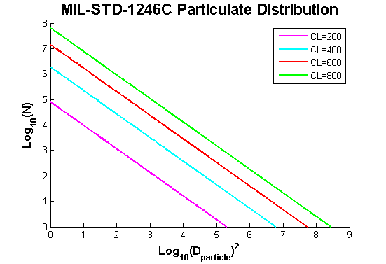
The functional form is:

where N is the number of particles having diameter greater than D microns at cleanliness level CL.
|
Uniform
|
|
Max. Dia
|
Maximum particle diameter in microns. For an unmodified MIL-1246C or IEST-STD-1246D distribution the maximum particle diameter in microns matches the specified cleanliness level, giving 1 particle of diameter CL per 0.1 m2.
|
400
|
|
Slope
|
Slope of the particulate distribution function. The default slope of 0.926 was determined empirically for freshly cleaned surfaces. Note, however, that you cannot simply change the slope of the distribution while keeping the same distribution function as this would result in an unrealistic percent area coverage (related to CL) for the surface(s).
|
0.926
|
|
CLevel
|
Cleanliness level that specifies 1 particle with diameter CLevel in microns per 0.1 m2. The cleanliness level sets the maximum particle size in the distribution. For example, a cleanliness level of 400 would be interpreted as 1 particle of diameter 400 microns per 0.1 m2.
CLevel <200 is a pristine surface.
Clevel = 600 is a visibly clean surface.
Clevel > 1000 is a visibly dirty surface.
|
|
|
|
Sampled Particle Size Distribution
|
Control
|
Inputs / Description
|
Defaults
|
|
Sampled Particle Size Distribution Specification
|
|
Density Func
|
Particle size distribution function. Choose Sampled.
|
Uniform
|
|
Data
|
Particle diameter, Particle density (number per um2). The particle density for the sampled distribution is not cumulative. The particle density represents the exact counts for the corresponding diameter.
Data can be read from a file by right mouse clicking in the spreadsheet area and selecting "Replace with Data From File". The *.dat file format consists of two header lines followed by rows of two column data, where the first data column is the particle diameter and the second data column is the density distribution. An example of this file format is shown below:
type mie_scatter_samples
format diameter density=sq_um
diam1 dens1
diam2 dens2
diam3 dens3
....
|
|
|
Note from the Description section of this help article that the BSDF for the Mie scatter model is determined by first calculating the phase function for an individual particle at each bin. The phase function for a single particle has significant ringing, which is washed out as the phase functions for each bin are accumulated to build up the full distribution. In this distribution the bin count N is equal to the number of data points provided and so, with the sampled distribution function, the user may note that the ringing persists when the number of samples is too few.
|
Application Notes
Wavelength dependence
The Mie model is weakly wavelength dependent. It is not generally necessary to enter additional Mie scatter models for all of the system wavelengths unless they span a large range.
Scatter in transmission and reflection
All scatter models describe the BSDF as measured over a maximum of 2p steradians. Both transmitted and reflected scatter can be modeled by specifying the two scatter directions simultaneously with the appropriate direction controls found under the Scatter tab in the Surface Dialog.
Surface Particle (Mie) Scatter TIS and plotting
Surface particle scatter is handled differently from other surface scatter models in FRED due to the fact that the Mie scattering is a volume effect. This fundamental difference necessitates calculation of the TIS for this model into 4p steradians rather than the 2p used with other models. If the model is in transmission, then you multiply the forward component by Surf Trans. If the model is in reflection, then the forward component is multiplied by Surf Refl. When plotting the BSDF for this model, the user may note differences in the TIS values reported for the 2D and 3D scatter plots. The 2D plot always shows the reflected BSDF and uses SurfRefl=1.0, so the TIS in the 2D plot will not be representative of the raytraced TIS. The 3D plot also shows the reflected BSDF but obeys the user-input value of SurfRefl, so the TIS will vary accordingly. A reliable method for reporting the TIS value of this scatter model is to use the ScatterTIS function.
Percent Area Coverage
The percent area coverage (PAC) is the fraction of the surface that is covered by particles, reported as the total particle projected area divided by the total surface area. This value is calculated by looping over each bin in the particulate distribution for the scatter model, calculating the projected area of the bin and multiplying by the number of particles in the bin, and then summing the results of all bins together. The PAC value is reported in the Detailed Report, which can be accessed by right mouse clicking on the scatter model in the object tree and selecting Detailed Report from the context menu.
Examples
The following examples show a series of 3-dimensional surface log plots of the normalized reflected BSDF (BRDF) as a function of scatter angle for 30 degrees angle of incidence.
Example 1 – Uniform Particle Size Distribution
The Mie scatter parameters are: Wavelen = 0.5 microns, Ref Index = 1.5, Imag Index = 0, Maximum Particle Size = 400 microns, Minimum Particle Size = 1 micron, Density = 0.1 particles per square micron. For a large range of particle sizes, this scatter model is close to Lambertian.
.gif)
Example 2 – Gaussian Particle Size Distribution
The Mie scatter parameters are: Wavelen = 0.5 microns, Ref Index = 1.5, Imag Index = 0, Maximum Particle Size = 400 microns, Minimum Particle Size = 1 micron, Mean Particle Size = 10 microns, Standard Deviation = 1 micron, Density = 0.1 particles per square micron.
.gif)
Example 3 – MIL-1246C Particle Size Distribution
The Mie scatter parameters are: Wavelen = 0.5 microns, Ref Index = 1.5, Imag Index = 0, Maximum Particle Size = 400 microns (= Level 400).
.gif)
Related Topics
ABg – for polished surface scatter
Binomial - plane symmetric case of general Polynomial
Extended Harvey-Shack - shift variant form of the Harvey-Shack model
Extended Scripted - User-defined scattering function that allows manipulation of the scattered rays' polarization state
Flat Black Paint – specify Total Integrated Scatter (TIS)
Harvey-Shack – for polished surface scatter
K-Correlation – analytic PSD
Lambertian – for diffuse scatter
Phong – cosn from specular
Polynomial - General polynomial with diffuse and Lorentzian component
Scripted - User-defined scattering function
Tabulated BSDF – measured BSDF data
Tabulated PSD – measured PSD data
References
Bohren, C. and Huffman, D., 1983. Absorption and Scattering of Light by Small Particles. New York: Wiley.
|
Copyright © Photon Engineering, LLC
|
|