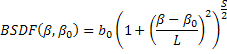
The Harvey-Shack model is linear shift-invariant with respect to incident angle and describes surface scatter from smooth optical surfaces over 2p steradians ( roughness sRMS << l). The mathematical form of the modified three term Harvey model is given by:
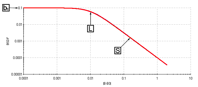
The physical interpretation of the three terms, L, b0, and S, is provided in the context of the b - b0 plot below: L - 'Knee' of the curve, typically between 0.0001 and 0.01 radians from specular b0 - Peak of the curve at |b-b0| = 0 S - Slope of the curve, typically between -0.5 and -2 (S < -2.5 is "super-polished")
This feature can be accessed by selecting Harvey-Shack (polished surface scatter) as the Scatter Type in the Create a new scatter model dialog box.
The Harvey-Shack model is linear shift invariant, which means that the BSDF depends only on the difference between the sine of the specular angle (b0) and the sine of the scattered angle (b). The angles b and b0 are always taken in the plane of the incident ray and are measured relative to the surface normal.
The relative scattered ray power in the specular direction (b-b0 = 0) is b0 multiplied by the projected solid angle in the specular direction. This product cannot exceed unity for a 100% scattering surface in order to obey conservation of energy.
The total integrated scatter (TIS) can be calculated from the following relationship when the RMS surface roughness, srms, is much less than l:
For a mirror, Dn = 2, indicating that mirrors scatter more than refractive optics in the visible range. The TIS is also calculated by integrating the BSDF, which gives the following relations for the Harvey model:
It is therefore possible to make reasonable assumptions for L and S and then solve for b0 to give the same TIS calculated from the RMS roughness. For example, suppose that a mirror surface has a 50 Angstrom RMS roughness with visible light at l = 0.5 um. The TIS calculated from the surface roughness is 0.015791. Without knowing anything further about the surface, it is assumed that S = -1.5 and L = 0.01 radians. Solving for the calculated TIS gives b0 = 1.396225 sr-1, completing the Harvey model definition.
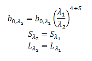
The Harvey-Shack model is wavelength invariant, but a non-rigorous scaling law proposed by Harvey can be used with caution when the ratio of the wavelengths (l1/ l2) is between 1/3 and 3.
Note in the equations above that only the b0 parameter scales. As the value of S is typically on the order of -2, it is often assumed that the scaling factor is simply the ratio of the wavelengths squared.
Scatter in transmission and reflection All scatter models describe the BSDF as measured over a maximum of 2p steradians. Both transmitted and reflected scatter can be modeled by specifying the two scatter directions simultaneously with the appropriate direction controls found under the Scatter tab in the Surface Dialog.
Multiple scatter models can be attached to the same surface. The scatter direction controls are then imposed on every attached model.
The following examples show a series of line plots of the Harvey-Shack BSDF as a function of scatter angle for specular angles of 0, 30, 45, 60, and 89 degrees. To illustrate the effect that changing L and S have on the scatter distribution, it is helpful to look at the function in log space. Each pair of plots to follow will show the angle space plot (as above) and its corresponding large angle specular log space plot. The ordinate axes for the log space plots are BSDF on the Y-axis, and |B-B0| on the X-axis.
The Harvey-Shack scatter parameters are b0 = 0.1, L = .01, and S = -1.5.
The Harvey-Shack scatter parameters are b0 = 0.1, L = .01, and S = -2.5. Changing the value of S from –1.5 to –2.5 causes the large angle scatter to fall off more rapidly.
The Harvey-Shack scatter parameters are b0 = 0.1, L = .001, and S = -1.5. Changing the value of L from .01 to .001 shifts the roll-off angle closer to specular, which has the effect of directing more of the scattered light into the specular direction. This also attenuates large angle scatter.
ABg – for polished surface scatter Binomial - plane symmetric case of general Polynomial Extended Harvey-Shack - shift variant form of the Harvey-Shack model Extended Scripted - User-defined scattering function that allows manipulation of the scattered rays' polarization state Flat Black Paint – specify Total Integrated Scatter (TIS) K-Correlation – analytic PSD Lambertian – for diffuse scatter Phong – cosn from specular Polynomial - General polynomial with diffuse and Lorentzian component Scripted - User-defined scattering function Surface Particle (Mie) – for particulate contamination Tabulated BSDF – measured BSDF data Tabulated PSD – measured PSD data
|
||||||||||||||||||||||||||||||||||||||||||||||||||||||
.png)
.gif)
.gif)
.gif)
.gif)
.gif)
.gif)