The Gaussian Diffuse model is linear shift-invariant with respect to incident angle and describes a Gaussian BSDF function in angular space. This model is intended to be used as an approximation to real scatter for numerical ease and/or computational efficiency. The Gaussian Diffuse model is capable of exhibiting anisotropic scatter. The mathematical form is given by:
Where: g0 - Peak of the Gaussian at |b-b0| = 0 σa - Sine of the angle representing one standard deviation in the 'a' direction ( |b-b0| ≈ 0.63g0 ) σb - Sine of the angle representing one standard deviation in the 'b' direction ( |b-b0| ≈ 0.63g0 ) Pa - Super Gaussian factor in the 'a' direction Pb - Super Gaussian factor in the 'b' direction
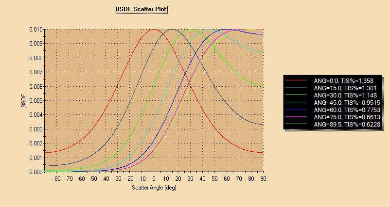
The plot below shows the BSDF of a symmetric Gaussian defined with σa = σb = 0.5 [i.e. 30 degrees], Pa = Pb = 1 and g0 = 0.01:
Note that for anisotropic scatter the 2D scatter charts will plot the BSDF in the plane of the 'b' direction only. Instead the 3D scatter chart can be used to see the anisotropic Gaussian scatter:
This feature can be accessed by selecting Gaussian Diffuse as the Scatter Type in the Create a new scatter model dialog box.
The Gaussian Diffuse model is linear shift invariant, which means that the BSDF depends only on the difference between the sine of the specular angle (b0) and the sine of the scattered angle (b). The angles b and b0 are always taken in the plane of the incident ray and are measured relative to the surface normal.
The relative scattered ray power in the specular direction (b-b0 = 0) is b0 multiplied by the projected solid angle in the specular direction. This product cannot exceed unity for a 100% scattering surface in order to obey conservation of energy.
The Gaussian Diffuse model is wavelength invariant.
Scatter in transmission and reflection All scatter models describe the BSDF as measured over a maximum of 2p steradians. Both transmitted and reflected scatter can be modeled by specifying the two scatter directions simultaneously with the appropriate direction controls found under the Scatter tab in the Surface Dialog.
Multiple scatter models can be attached to the same surface. The scatter direction controls are then imposed on every attached model.
ABg – for polished surface scatter Binomial - plane symmetric case of general Polynomial Extended Harvey-Shack - shift variant form of the Harvey-Shack model Extended Scripted - User-defined scattering function that allows manipulation of the scattered rays' polarization state Flat Black Paint – specify Total Integrated Scatter (TIS) Harvey-Shack - for polished surface scatter K-Correlation – analytic PSD Lambertian – for diffuse scatter Phong – cosn from specular Polynomial - General polynomial with diffuse and Lorentzian component Scripted - User-defined scattering function Surface Particle (Mie) – for particulate contamination Tabulated BSDF – measured BSDF data Tabulated PSD – measured PSD data
|
||||||||||||||||||||||||||||||||||||||||||||||||||||||||||||||||||