This tutorial discusses discusses how to use FRED to accurately model the coupling from a ball-lens capped semiconductor laser diode to a single mode fiber - an optical system common in optical fiber communication applications. This model demonstrates FRED’s capability to propagate coherent fields, its accurate astigmatic laser diode source type and its ability to calculate fiber coupling efficiency. Additionally, longitudinal, horizontal and angular alignment sensitivity of the fiber position is studied via embedded scripts. Through out this tutorial, the user will be referred to other sections of the help system for further discussion on specific topics.
The accompanying FRED file for this tutorial can be found in <install dir>\Resources\Samples\Coherence\systemFiberCoupler.frd.
The semiconductor laser diode used in this tutorial is the Mitsubishi ML725C8F, which is an InGaAsP / InP multiple quantum well (MQW) laser that operates at 1310nm wavelength. The Mitsubishi source specifications define the output beam as astigmatic with beam divergence angles in x and y defined as 25 and 30 degrees respectively (full 1/e width of the far field power profile). No mention is made of any offsets in the focal positions in x and y, so they are assumed to be coincident and at the source waist location. This laser diode source is modeled in FRED using the Laser Diode Beam (coherent) type of Source Primitive.
Note that in the settings for the Laser Diode Beam source, the divergence angles are defined by the full width at the 1/e2 power point. Since the vendor specification supplies the full width of the 1/e power point, the angles provided by the manufacturer are multiplied by a factor of sqrt(2) as shown in the above dialog.
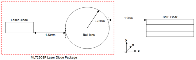
The schematic for the ball-lens capped laser diode to fiber system is shown below. The 1.5mm diameter ball lens is part of the Mitsubishi laser diode package and is positioned 1.88mm from the emitting surface of the laser diode.
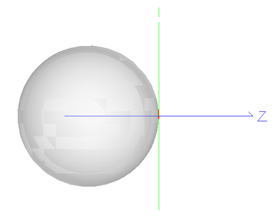
The ball-lens is created in FRED using a spherical Element Primitive where, for convenience, the global origin is chosen to be where the output surface of the ball lens intercepts the optical axis.
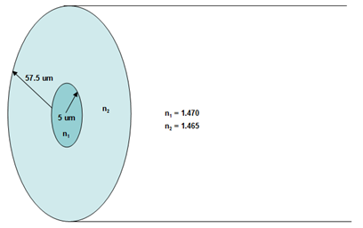
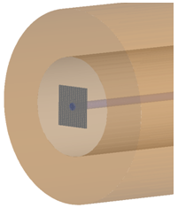
The single mode fiber (SMF) used in the model is located 1.9 mm from the global origin and has dimensions (defined in the figure below) based on values that are typical for a SMF. The fiber core has radius 5 microns and is surrounded by a cladding that is 125 microns across. The refractive index values for the core and the cladding are 1.465 and 1.47 respectively, giving a refractive index difference of 0.36%. Additionally, an absorbing coating surrounding the fiber is included in the model.
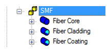
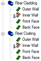
The fiber is defined in FRED as a Subassembly containing multiple Element Primitives – a cylinder for the core, and pipes for both of the cladding and coating:
Note that inside wall of the “Fiber Cladding” pipe coincides exactly with the outer wall of the “Fiber Core” cylinder. To model this correctly the user needs to manually set the Inner Wall of both the cladding pipe to be not traceable. Failure to do this will lead to raytrace errors as we have two surfaces located at exactly the same position in space and with two different sets of materials. The same needs to be done for the Inner Wall of “Fiber Coating.”
In this model the fiber coating is considered to be absorbing and has Halt All raytrace control. All other surfaces are uncoated.
FRED calculates the fiber coupling efficiency as described in the Fiber Coupling Efficiency help topic. Therefore, to calculate the fiber coupling accurately an Analysis Surface needs to be located just behind the fiber entrance to ensure that the reflection coefficient at this interface is correctly taken into account (as shown below). It is important that the Analysis Surface is larger than the expected mode field diameter (MFD) of the fundamental mode so as to perform an accurate overlap integral. It is also important to be aware that the accuracy of this numerical integration is dependent on the number of divisions in the Analysis Surface. In this case, 251 x 251 pixels on a 50um wide Analysis Surface is deemed sufficient.
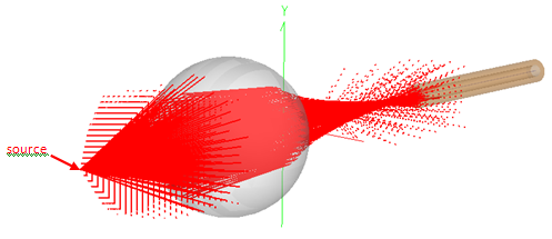
The 3D rendering below shows the fiber coupling model traced with 129 x 129 samples in the source.
The value returned by FRED’s fiber coupling efficiency calculation is the overlap fraction between the two field profiles; it does NOT take into account the power of the incident field. Therefore understanding how much power is coupled to the mode must be done in two steps: 1. Determine the amount of power (P) at the Analysis Surface by performing an Irradiance calculation. 2. Determine the CE fraction from the fiber coupling efficiency analysis.
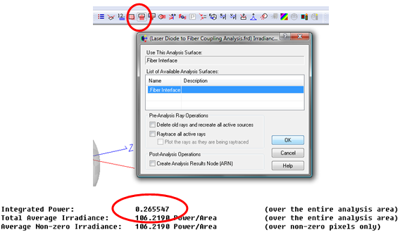
The amount of power that is coupled to the fiber mode is given simply by P * CE. After tracing the rays from the source, the fraction of source power that reaches the Analysis Surface behind the fiber interface is displayed in the Output Window when we calculate the Irradiance.
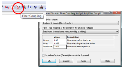
From the output above, 26.55% of the source power reaches the Analysis Surface (assuming a starting source power of 1). In order to determine the coupling to the fiber mode, FRED’s Fiber Coupling Efficiency analysis is used. Note that the fiber index values and the core radius have to be entered explicitly here.
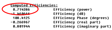
After clicking OK in the fiber coupling efficiency dialog, the analysis results are displayed in the output window.
The coupling efficiency is 71.44%. Therefore in this system the total coupled power percentage is 71.44% * 26.55% = 19.0%. The ML725C8F laser diode source operates at 5 mW, therefore in this configuration the fiber will be transmitting a signal of just under 1 mW.
Understanding the fiber alignment sensitivity is critical for gauging the design tolerances and, consequently, the feasibility of this laser diode / fiber package. This can be done quite simply using FRED’s scripting functionality. There are six embedded scripts associated with this FRED document:
The two sets of scripts are similar to each other; the "to EXCEL" scripts display plot results in EXCEL using COM while the second set plots the script results directly in a FRED chart window using the 2D chart scripting commands. The following discussions refer to the "to EXCEL" versions of the scripts.
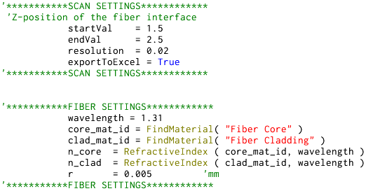
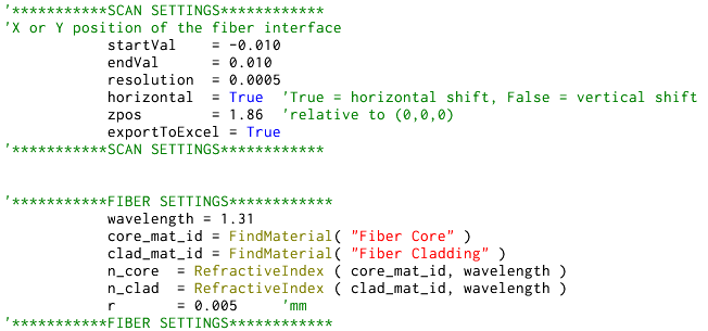
Longitudinal alignment sensitivity At the top of the "Distance Scan to EXCEL" script the user inputs the start and end positions of the fiber and the resolution of the scan that they wish to run. The boolean "exportToExcel" is set to True if the user wishes FRED to print the data to a Microsoft Excel spreadsheet and plot a graph automatically. Just under this the fiber parameters are defined. These are used for the fiber coupling efficiency calculation only.
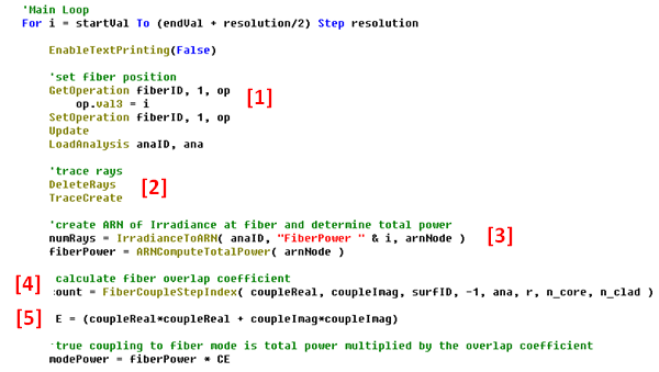
After the headers are printed, the main loop of the script starts. This is a For loop that will step by step alter the position of the fiber - [1], trace the rays - [2], calculate the Irradiance & determine the total power - [3], calculate the fiber coupling coefficient - [4], and finally calculate the mode power - [5].
Note that the function FiberCoupleStepIndex returns two values – “coupleReal” and “coupleImag.” The coupling efficiency is a complex quantity and these variables are the real and imaginary coefficients. The coupling power is determined by:
CE = coupleReal2 + coupleImag2
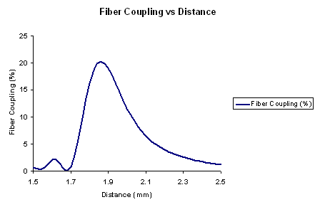
The figure below shows the results for varying the distance from the ball lens to the fiber from 1.5 mm to 2.5 mm.
The manufacturer of the laser diode, Mitsubishi, specifies that the maximum fiber coupled power is 0.8 mW (16% efficiency) at a position of 1.9 mm from the ball lens. FRED calculates a slightly larger value for the coupling, but this is attributed to the fact that the coupling is very sensitive with respect to the fiber mode size and index and the exact details of the fiber used by Mitsubishi are not given.
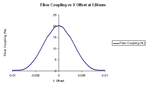
Horizontal Alignment Sensitivity The script “Lateral Offset Scan to EXCEL” is very similar to previous longitudinal scan, except that the user defines the parameters as shown below with the resulting output.
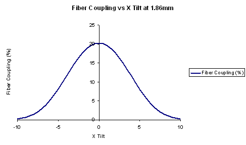
This script is also very similar to the previous scripts; here the user defines the angular range of the orientation. Note that this script tilts the fiber in the horizontal direction only, not at an arbitrary angle. The resulting output is shown below.
|
.png)