Diffraction gratings are implemented as an attribute on a surface characterized by a local grating frequency at the point of intersection and a corresponding diffraction efficiency that may depend on wavelength, order, polarization, and incident direction (sidedness). During raytracing, a vector form of the grating equation is used to represent the effect of the grating structure; at no point is the physical structure of the grating represented by the geometry. As many diffraction orders will be generated as are defined by the user-supplied diffraction efficiency data, as long as the requested order is not evanescent.
A diffraction grating is implemented through two specifications found on the Grating tab of a surface dialog:
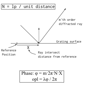
The grating type specifies the phase profile applied to the surface so that when a ray interacts with the surface, the appropriate amount of phase is added to the ray in order to model the grating effects. The phase (and path length) additions are calculated as shown in the diagram below.
The following Grating Types are available to be specified: •Linear (Evenly spaced linear grating lines) •Two point exposure holographic optical element •Two source user-recorded holographic optical element
The diffraction efficiency is specified either as a lookup table or as a volume hologram calculation on the surface's Grating tab. When a ray interacts at a surface having a grating property, the wavelength and incident polar and azimuthal angles, and polarization are used to determine the appropriate relative power for each requested diffraction order in the efficiency table. Note that the resulting diffracted rays are additionally operated on by the associated surface's specular coating properties.
The following diffraction efficiency table types are available to be specified: •Simple efficiency table (wavelength and diffraction order) •Full efficiency table (wavelength, diffraction order, polar and azimuthal angles, polarization, reflection and/or transmission) •Volume hologram efficiency (wavelength, AOI, and polarization, reflection and/or transmission)
This feature can be accessed by selecting the Grating tab in a surface dialog.
Gratings, Raytrace Controls and Parentage When a ray intersects a grating surface with specular ancestry level below the cutoff value set by the grating surface's raytrace property (ex. ray ancestry = 1, raytrace control specular ancestry = 2), all non-evanescent diffraction orders will be allowed to propagate away from the grating. In this case, the parentage is governed by the raytrace property (highest power, transmitted highest power, reflected highest power, monte-carlo). However, if a ray intersects a grating and has a specular ancestry level equal to the specular ancestry cutoff value set by the grating surface's raytrace property (ex. ray ancestry = 1, raytrace control specular ancestry = 1), then FRED will attempt to propagate only one of the defined diffraction orders subject to the following behaviors:
•For efficiency table specifications (simple and full), the diffraction order selected for propagation is the order in the first column of the table. For full efficiency tables, the internal table ordering can be viewed by right mouse clicking on the grating surface and selecting the Detailed Report option. •For the volume hologram efficiency specification, whichever component is selected as Order 0 will be selected for propagation. •If the selected order is evanescent (or otherwise does not meet power thresholds set by the raytrace property) then the user will observe that no ray is propagated away from the grating. If the selected order is not evanescent, then the user should observe that this order propagates away from the grating and will maintain the same ancestry level as the incident ray.
This behavior regarding the ancestry level is unique to grating surfaces. Due to the fact that gratings may have many diffracted orders, it would be inefficient for FRED to generate all diffracted rays, establish which order maintains the parent ancestry level status and then have to throw away the remaining rays due to ancestry level cutoffs (this would have to be done every time a ray intersected the grating!).
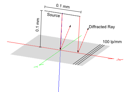
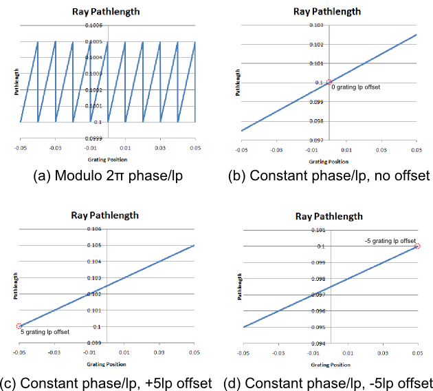
Amount of phase to add per grating line The default grating settings add phase continuously between line pairs but modulo 2p across the entire grating, resetting the phase when crossing into a new line pair. For some applications, the desired behavior is that phase is added continuously across the entire grating. The options "Add modulo 2p phase per grating line" and "Add full 2p phase per grating line" allow the user to toggle between these two modes of operation. The additional specification "Grating line offset (number of grating lines)" allows the user to specify the zero phase point in the grating with respect to the surface origin when operating in the continuous phase mode. Consider the following system, where a line source perpendicular to the ruling direction is incident on a 100 lp/mm linear grating. The source is located 0.1mm from the grating along the surface normal and has a 0.1mm width, allowing rays to sample 10 line pairs across the grating.
After tracing the source rays to the reflective grating, each ray is queried for its position and pathlength and the results are written out and plotted. The plots below show the path length across the 0.1mm section of the grating surface using the modulo 2p option and the continuous phase option with different line pair offsets. For this configuration, the zero phase point is indicated by the position whose pathlength equals the distance from the source to the grating (0.1mm). In configuration (a) the grating phase is applied modulo 2p so that the phase is continuous between grating line pairs but resets at each new line pair. In configuration (b) the phase is applied continuously across the grating with zero lp offset so that the 0 phase point is at the surface origin (indicated by the 0.1 pathlength). In configuration (c) the phase is applied continuously across the grating with a +5 lp offset, indicating that the surface origin is +5 lp away from the zero phase point. In configuration (d) the phase is applied continuously across the grating with a -5 lp offset, indicating that the surface origin is -5 lp away from the zero phase point.
The table below relates the above information to the controls found at the bottom of the Grating tab on the surface's dialog in the section, "Amount of phase to add per grating line (usually modulo 2PI):
Primary and Secondary Efficiency Tables The diffraction efficiency tables determine the distribution of power over the specified diffraction orders. For transmissive gratings, the efficiency of each order is dependent on whether the ray is propagating from a low index to a high index or visa versa. To account for the dependency on the direction of a ray relative to the grating surface (i.e. from which side of the grating the ray is incident on), FRED has the ability to use up to two diffraction efficiency tables. The behavior of the efficiency tables, called the Primary and Secondary tables, obeys the following rules: •If both the primary and secondary efficiency tables are set to "none", then no diffraction grating effects will be applied. •If one of either the primary or secondary efficiency tables (but not both) are set to "none", then the efficiency table that is not "none" will be applied regardless of the direction of the incident ray. This option should be used with reflection gratings or with transmission gratings where the user does not care (or does not know) about the dependency on efficiency with regard to sidedness. •If both the primary and secondary efficiency tables are not "none" then the primary efficiency table will be applied when the dot product of the incident ray and the local surface normal is positive. The secondary efficiency table will be applied when the dot product of the incident ray direction and the local surface normal is negative. •For planar gratings, the local surface normal is always in the +Z direction. So, the primary efficiency table will be applied when the incident ray direction has a +Z component relative to the surface's coordinate system and the secondary table will be applied when the incident ray direction has a -Z component relative to the surface's coordinate system. •There is no requirement that the primary and secondary efficiency tables use the same table type. For example, the primary table could use the "Simple Efficiency Table" model and the secondary table could use the "Full Efficiency Table" model.
Specification of the primary and secondary efficiency tables is implemented by first toggling the appropriate radio button in the diffraction efficiency portion of the Grating tab on a surface dialog and then choosing the appropriate table type from the drop-down list below it.
The grating attribute of a surface with a birefringent material assigned to it will be ignored. In order to compute a diffracted ray direction, the refractive index of the incident and outgoing rays must be known. However, for birefringent materials, the refractive index depends on the ray direction. For the case of Snell's Law, a ray's refractive index in a uniaxial birefringent material is computed using an iterative algorithm published by Chipman et. al. Photon Engineering is unaware of a published algorithm for computing diffracted rays immersed in a birefringent media.
|
.png)