|
Description
The full diffraction efficiency table can interpolate power and phase (radians) efficiency values and is primarily designed to support the output from grating analysis programs such as GSolver. This implementation of the diffraction efficiency table includes a dependence on wavelength and incident polar and azimuthal angles, distinguishes between diffraction orders in reflection and transmission, and can optionally include S and P polarization efficiencies and polarization cross-coupling. No extrapolation is performed on the data when the incident ray's wavelength or angle lies outside the bounds of the sampled data; the efficiency data from the closest sample point will be applied.
After an efficiency file has been loaded into the dialog, summary information is provided back to the user regarding the number of entries and value ranges found for each parameter. After applying the changes, the user can get an exact listing of the efficiency table data in the output window by right mouse clicking on the surface on the object tree and selecting "Detailed Report" from the menu options.
Because diffraction orders are specular operations, the surface coating definition will apply to the ray powers on top of the grating efficiency table value. The user should create a fictitious sampled coating with R=1 and T=1 to be applied to the grating surface so that the ray power is completely determined by the full efficiency table.
The interpolation of the efficiency table occurs over wavelength, incident angle, and azimuthal angle (for each polarization component, if specified). The eight nearest sample table values for each of wavelength, incident angle, and azimuthal angle define the corners of a hypercube in wavelength, incident angle and azimuthal angle space. These eight corners are labeled E000, E100, E010, E001, E110, E101, E011 and E111. The (wavelength, incident angle, azimuthal angle) point in the hypercube space is located inside the cube and the normalized coordinates of this point is denoted as (a,b,c). For example, (0,0,0) is the corner with efficiency value E000, and (1,1,1) is the corner with efficiency value E111, etc. A tri-linear interpolation in this space is performed and is mathematically equivalent to the following:
E(a,b,c) = (1-a)(1-b)(1-c)E000 + a(1-b)(1-c)E100 + (1-a)b(1-c)E010 + (1-a)(1-b)cE001 + ab(1-c)E110 + a(1-b)cE101 + (1-a)bcE011 + abcE111
From the scripting language, the GetInterpolatedDiffractEfficiency() function can be used to query a grating surface with the Full efficiency table specification for its interpolated efficiency values, which can be useful for debugging and verification.
Navigation
The Full efficiency table specification can be accessed from the Grating tab of a surface dialog. The section on the right hand side of the dialog corresponds to the diffraction efficiency specification for the grating. In the drop-list box, select "Full efficiency table".
.png)
Controls
|
Control
|
Inputs / Description
|
Defaults
|
|
File Name
|
Use the Select button to open a file browser and select an ASCII file containing the diffraction efficiency data. After reading the file, the data is stored internally to the grating surface. There is no requirement that the file is accessible to FRED thereafter.
|
no file name selected
|
|
File Format
The full diffraction efficiency table data is loaded from an ASCII file consisting of a single header line indicating the quantity in each column followed by an arbitrary number of rows containing the values for each column.
Specification of the column headers:
Reflected Orders, Power efficiency: numeric value followed by "R", ex. "-1R" indicates the column corresponds to power efficiency in the minus 1 order in reflection
Reflected Orders, Phase efficiency: numeric value (in radians) followed by "r", ex. "-1r" indicates the column corresponds to phase efficiency in the minus 1 order in reflection
Transmitted Orders: numeric value followed by "T", ex. "2T" indicates the column corresponds to the power efficiency in the plus 2 order in transmission
Transmitted Orders, Phase efficiency: numeric value (in radians) followed by "t", ex. "2t" indicates the column corresponds to phase efficiency in the plus 2 order in transmission
Wavelength: keyword "lambda"
Polar Angle: keyword "theta"
Azimuth Angle: keyword "phi"
Polarization (optional): keyword "type"
The following efficiency file format rules apply:
•The "type" column is optional. If the "type" column is not included, the behavior of the grating is scalar.
•Phase efficiency values are given in radians.
•Wavelength values are given in microns.
•Polar and Azimuth angles are given in degrees.
•Efficiency values for all unique polar and azimuthal angle sample points in the data file should be specified, otherwise those values will be assumed to be zero. Failure to specify data values at each unique polar, azimuthal angle pair will result in zeros during interpolation.
•If phase efficiency columns are not present, they are assumed to be zero.
•If only an SS polarization component is present, a PP component is assumed with the same values.
•If SP and PS polarization components are not present, they are assumed to be zero.
•Unrecognized column headers are ignored.
•Column order does not matter.
•Row order does not matter.
•FRED will update the polarization components of the ray as defined by the efficiency file. This does not guarantee correctness. The user bears the responsibility for providing FRED with data that is physical and reasonable.
•There is no standard convention for +/- diffraction orders in optical software. The user bears the responsibility for confirming that rays leaving the grating have the proper angle relative to the optical design.
A text file can be generated directly from GSolver by saving out the data from the Results tab after an analysis run. This file can be read into the full diffraction efficiency table after correcting for azimuthal angle conventions.
An optional file header line related to the interpolation of phase values near a +/- phase boundary can be placed at the start of the file using the format
phasetol N
where N is a value in radians (ex. 0.5). See the phase interpolation notes below.
Scalar efficiency file format example
The example below shows a scalar efficiency file which designates the power efficiency for two orders in reflection (-1 and +1), one order in transmission (+1) with a dependence on wavelength and polar angle (theta). There is no dependence on azimuthal angle or polarization and no phase efficiency data is provided. A phase unwrapping tolerance is specified in the first line of the file (see phase interpolation notes below).
|
phasetol 0.5
|
|
1R
|
-1R
|
1T
|
lambda
|
theta
|
phi
|
|
0.000353
|
0.000353
|
0.204369
|
0.4
|
0
|
0
|
|
0.000733
|
0.000174
|
0.193368
|
0.4
|
10
|
0
|
|
0.004427
|
0.000228
|
0.216915
|
0.4
|
20
|
0
|
|
0.012565
|
0.000549
|
0.275482
|
0.4
|
30
|
0
|
|
0
|
0.001428
|
0.294326
|
0.4
|
40
|
0
|
|
0
|
0.005586
|
0.060179
|
0.4
|
50
|
0
|
|
0
|
0.0124
|
0
|
0.4
|
60
|
0
|
|
0
|
0.010568
|
0
|
0.4
|
70
|
0
|
|
0
|
0.004716
|
0
|
0.4
|
80
|
0
|
|
0.005025
|
0.005025
|
0.142478
|
0.5
|
0
|
0
|
|
0.007395
|
0.004288
|
0.153625
|
0.5
|
10
|
0
|
|
0.006145
|
0.004295
|
0.180435
|
0.5
|
20
|
0
|
|
0
|
0.005031
|
0.214635
|
0.5
|
30
|
0
|
|
0
|
0.007089
|
0.072364
|
0.5
|
40
|
0
|
|
0
|
0.008058
|
0
|
0.5
|
50
|
0
|
|
0
|
0.005311
|
0
|
0.5
|
60
|
0
|
|
0
|
0.002667
|
0
|
0.5
|
70
|
0
|
|
0
|
0.001355
|
0
|
0.5
|
80
|
0
|
Vector efficiency file format example #1
The example below shows a vector efficiency file which designates the power efficiency for two orders, +1 in transmission and +1 in reflection, with no dependence on wavelength or incident angles. No phase efficiency values are defined. Each row in the table corresponds to one of the four polarization terms used in calculating the efficiencies in S and P with cross-coupling included. There are no cross-component contributions in this example definition.
|
1T
|
1R
|
lambda
|
theta
|
phi
|
type
|
|
0.3
|
0
|
0.5
|
0
|
0
|
SS
|
|
0.03
|
0
|
0.5
|
0
|
0
|
PP
|
|
0
|
0
|
0.5
|
0
|
0
|
SP
|
|
0
|
0
|
0.5
|
0
|
0
|
PS
|
Vector efficiency file format example #2
The example below is an extension of the previous table, where columns for phase efficiency, "1t" and "1r", have been added.
|
1T
|
1t
|
1R
|
1r
|
lambda
|
theta
|
phi
|
type
|
|
0.3
|
0
|
0
|
0
|
0.5
|
0
|
0
|
SS
|
|
0.03
|
0
|
0
|
0
|
0.5
|
0
|
0
|
PP
|
|
0
|
0
|
0
|
0
|
0.5
|
0
|
0
|
SP
|
|
0
|
0
|
0
|
0
|
0.5
|
0
|
0
|
PS
|
Vector efficiency file format example #3
The example below shows a vector efficiency file formatted with power efficiency values specified in six orders (+1, +2 and +3 for transmission and reflection) and phase efficiency specified in the +1 reflection order. There is a variation with polar and azimuth angle but the wavelength is constant. Only the 90 degree azimuth sample points contain non-zero cross-component polarization values.
|
3R
|
2R
|
1R
|
3T
|
2T
|
1T
|
1r
|
lambda
|
theta
|
phi
|
type
|
|
0.3001
|
0.2001
|
0.1001
|
0.3002
|
0.2002
|
0.1002
|
0.001
|
0.5
|
0
|
0
|
SS
|
|
0.3501
|
0.2501
|
0.1501
|
0.3502
|
0.2502
|
0.1502
|
0.002
|
0.5
|
0
|
0
|
PP
|
|
0
|
0
|
0
|
0
|
0
|
0
|
0
|
0.5
|
0
|
0
|
SP
|
|
0
|
0
|
0
|
0
|
0
|
0
|
0
|
0.5
|
0
|
0
|
PS
|
|
0.4001
|
0.3001
|
0.2001
|
0.4002
|
0.3002
|
0.2002
|
0
|
0.5
|
5
|
0
|
SS
|
|
0.4501
|
0.3501
|
0.2501
|
0.4502
|
0.3502
|
0.2502
|
0
|
0.5
|
5
|
0
|
PP
|
|
0
|
0
|
0
|
0
|
0
|
0
|
0
|
0.5
|
5
|
0
|
SP
|
|
0
|
0
|
0
|
0
|
0
|
0
|
0
|
0.5
|
5
|
0
|
PS
|
|
0.4001
|
0.3001
|
0.2001
|
0.4002
|
0.3002
|
0.2
|
0.006
|
0.5
|
5
|
90
|
SS
|
|
0.4501
|
0.3501
|
0.2501
|
0.4502
|
0.3502
|
0.25
|
0.007
|
0.5
|
5
|
90
|
PP
|
|
0.0041
|
0.0031
|
0.0021
|
0.0042
|
0.0032
|
0.0022
|
0.008
|
0.5
|
5
|
90
|
SP
|
|
0.0045
|
0.0035
|
0.0025
|
0.0046
|
0.0036
|
0.0026
|
0.009
|
0.5
|
5
|
90
|
PS
|
|
|
Efficiencies
|
After an efficiency file has been loaded, this entry lists the minimum and maximum efficiency values read from the file (ex. "Efficiency values from 0 to 0.975").
|
Efficiency values from 1 to 1
|
|
Orders
|
After the efficiency file has been loaded, this entry lists the number of orders found and their minimum and maximum values (ex. "3 order(s) from -1 to 1").
|
1 order(s) from 0 to 0
|
|
Wavelengths
|
After the efficiency file has been loaded, this entry lists the number of wavelengths and their minimum and maximum values (ex. "2 wavelength(s) from 0.5 to 0.6 microns").
|
1 wavelength(s) from n to n
|
|
Inc Angles
|
After the efficiency file has been loaded, this entry lists the number of incident angles found and their minimum and maximum values (ex. "5 incident angle(s) from 0 to 45 deg").
|
1 incident angle(s) from 0 to 0 deg
|
|
Azimuth Angles
|
After the efficiency file has been loaded, this entry lists the number of azimuth angles found and their minimum and maximum values (ex. "5 azimuthal angle(s) from -180 to 180 deg").
|
1 azimuthal angle(s) from 0 to 0 deg
|
|
CAUTION! No standard convention exists for constructing the local grating coordinate system which defines the azimuthal angle. In FRED, azimuthal angles are calculated on the range from -180o <= f <= 180o in the coordinate system shown below. The user bears responsibility for verifying the sign convention in the file being used to populate the efficiency table.
The diagram below shows the case of a ray incident on a linear grating with grating lines rotated by angle w relative to the surface's X axis. A local grating coordinate system is setup in the following way to calculate the azimuthal angle for the incident ray. The blue axes is the grating coordinate system and the red axes is the local surface coordinate system.
1. Zg = Grating normal
2. Xg = Grating vector direction
3. Yg = Zg x Xg
4. Incident ray direction is projected into the grating plane to get the Xg and Yg components, Rx and Ry
5. Azimuthal angle is calculated as Atan2(Rx,Ry)
As shown below, a ray is incident on the grating with polar angle q and the azimuthal angle is measured positive from Xg to Yg and negative from Xg to -Yg.
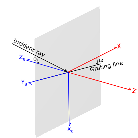
(Above) Formation of the grating coordinate system and incident ray with polar angle, theta
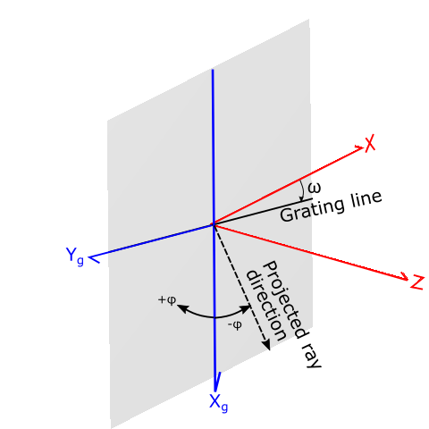
(Above) Calculation of the ray's azimuth angle, phi, by projection of the incident ray into the grating coordinate system
|
Polarization dependent diffraction efficiency
The complex amplitudes of the diffracted ray's output S and P polarization states, As’ and Ap’, are given by the matrix equation below. As and Ap are the complex amplitudes of the incident ray. Each of the four components, SS, PP, SP and PS, have the form, Sqrt(power_efficiency)*exp( +i * phase_efficiency), with the phase efficiency given in radians.
.png)
The SP and PS coefficients represent the cross-coupling between the S and P states. The S' polarization vector for the outgoing ray is perpendicular to the plane defined by the diffracted ray's direction vector and the surface normal, while the P' polarization vector is parallel to this plane.
The diffracted ray's flux is given by φ = |As’|*|As’| + |Ap’|*|Ap’|.
A procedure for verifying ray data
The complex nature of the Full efficiency table with dependencies on wavelength, polar and azimuthal angles, and polarization state can make it difficult to verify application of the efficiency data globally for an entire rayset. However, the following procedure can be used to verify application of the efficiency data on a ray-by-ray basis for the purposes of debugging and validation. If the user only wishes to check the interpolation of the grating data, then the GetInterpolatedDiffractEfficiency function can be used.
Step 1 - Idealized Behavior
The first step in this procedure is to establish the behavior of the diffracted rays in the idealized case for 100% efficiency (i.e. determination of As and Ap in the matrix construction above).
1. Configure the grating to use the Simple efficiency table option and configure the diffracted order to be evaluated with an efficiency of 1.0.
2. Perform a raytrace and then use the Tools > Reports > Ray Detail (for one ray) utility to retrieve the detailed ray data for the ray of interest.
3. From the detailed ray data in (2) above, retrieve the S and P direction vectors for the ray as well as the As and Ap complex amplitudes.
4. Calculate |As| and |Ap| as |A| = Sqr( Re{ }2 + Im{ }2 ) for each component.
5. Calculate the phase of each component, phi_s and phi_p, as Atan2(Re,Im) in radians.
Step 2 - Apply Diffraction Efficiency
The next step in this procedure is to apply the SS, PP, SP and PS efficiency components to the idealized ray data from Step 1.
1. From the efficiency file data, retrieve Axx * exp( i*phi ) for each component, where Axx = Sqrt(power_efficiency) and phi = phase_efficiency.
2. Calculate the quantities:
As' = ( |Ass|*exp( i*phi_ss ) )( |As|*exp( i*phi_s ) ) + ( |Asp|*exp( i*phi_sp ) )( |Ap|*exp( i*phi_p ) )
Ap' = ( |Aps|*exp( i*phi_ps ) )( |As|*exp( i*phi_s ) ) + ( |App|*exp( i*phi_pp ) )( |Ap|*exp( i*phi_p ) )
which expand to,
As' = { |Ass||As| cos( phi_ss + phi_s ) + |Asp||Ap| cos( phi_sp + phi_p ) } + i { |Ass||As| sin( phi_ss + phi_s ) + |Asp||Ap| sin( phi_sp + phi_p ) }
Ap' = { |Aps||As| cos( phi_ps + phi_s ) + |App||Ap| cos( phi_pp + phi_p ) } + i { |Aps||As| sin( phi_ps + phi_s ) + |App||Ap| sin( phi_pp + phi_p ) }
3. Normalize As' and Ap' by the magnitude, Sqr( Re{As')2 + Im{As'}2 + Re{Ap'}2 + Im{Ap'}2 ) to get the final As' and Ap'
4. The diffracted ray's flux is given by |As'|*|As'| + |Ap'|*|Ap'|, assuming the incident ray's flux is 1.0
Phase Interpolation
Interpolation of phase components during raytracing requires special handling near sample points with 2PI phase jumps. Consider two adjacent sample points, one defining a phase of +3 radians at a polar angle of 5 degrees and another defining a phase of -3 radians at a polar angle of 15 degrees. Interpolation of the phase between 5 and 15 degrees should wind around the phase circle passing through the +/-PI phase discontinuity. In a straight linear interpolation, however, the phase between 5 and 15 degrees would pass through zero phase going from +3 radians to -3 radians. A signature of this zero-phase interpolation effect can be the presence of unexpected artifacts in an irradiance or field distribution that track +/-PI phase discontinuity boundaries in a phase efficiency map.
By default, if two adjacent data points have a phase difference within 0.5 radians of 2PI, FRED will automatically add +2PI or -2PI radians to one of the points so that the adjusted phase difference is less than 0.5 radians and the interpolated value does not pass through zero phase.
If a custom phase tolerance value (0.5 radians unless otherwise specified) is desired, the following header line can be optionally specified in the first row of the efficiency file:
phasetol n
where n is the phase tolerance value in radians (ex. phasetol 0.25).
Related Topics
Gratings Overview
Grating Types
Simple Efficiency Table
Volume Hologram Efficiency
|
Copyright © Photon Engineering, LLC
|
|