Analysis planes are used to evaluate ray distributions on surfaces or sources and are required for use of the analysis functions. Analysis planes do not interact with rays during a raytrace, rather, they contain one or more ray filters used select a subset of rays for analysis. Rays can be filtered and analyzed at any time and location after they are created in the system, before or after raytracing.
Analysis Planes can only be used in conjunction with surface or source entities, though more than one analysis plane can be attached to a surface or source.
Analysis surfaces can be created in the following ways: •Menu > Create > New Analysis Surface •Right mouse click on the Analysis Surfaces(s) folder in the tree view and select the option ‘New Analysis Plane’ •Right mouse click on a surface node in the object tree and select the option, “Auto Create and Attach an Analysis Surface” •Toolbar button: •Ctrl + Alt + N
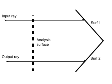
A common misconception in the use of analysis surfaces is that they intercept rays during the raytrace and will therefore include results from multiple ray passes through the geometric position of the analysis plane. However, this is not the case. Consider the image below where an analysis surface is located between a source input ray and an output ray after retro-reflection.
In this case performing an analysis (eg. irradiance) after the raytrace would show only results from the output ray and will not include the "first" pass by the input ray. The reason for this is that each ray has an association with a surface or source entity, which in general is the last surface of intersection. So, when the analysis surface filters the rays it sees that the output ray is associated with Surf 2 and the ray is projected along its current direction until it intersects the analysis surface, where the calculation is performed.
If a calculation is desired such that the results include both the "first" and "second" passes of the input and output rays, respectively, then two separate analyses must be performed and the results combined. For this case the following steps should be taken to build a composite irradiance calculation:
The resulting analysis should include both calculations from the input and output rays. These steps can be generalized for more complex geometries and composite analyses.
Positional and Angular Analysis An analysis plane may be used for both positional and angular (intensity) analysis, though it is recommended to have one analysis plane for each type. For positional analysis, the size of the analysis plane is given in system units. When Interpret Min / Max as Angles (degrees) is checked the current values in the Min / Max text boxes are interpreted as the X and Y direction cosines measured from the surface normal. Values on the range -1 to 1 are therefore interpreted as - / + 90 degrees. Once the user has toggled this check box values can be entered as degrees.
Sizing Analysis Planes for Coherent Calculations Allowing FRED to auto-size the analysis plane in coherent calculations usually results an undersized analysis plane because the algorithm is based on the geometrical raytrace rather than the extent of the field. It is suggested that the user set the size manually when performing coherent calculations.
Analysis planes are not required to be positioned coincident with a surface or source entity. If the analysis plane is displaced from an entity of analysis interest, FRED simply projects the rays from the entity along their current trajectories until the intersect the displaced analysis plane. When an analysis plane is attached to a source or surface FRED moves the analysis plane to be coincident with the local origin of the surface or source and imposes a ray selection filter that tells FRED to consider only the rays currently associated with that surface or source.
At the conclusion of any analysis operation a host of information regarding the current analysis is printed to the output window. This information is extremely valuable in determining the characteristics of the analysis results and also provides error messages and warnings.
Example 1 – Attach an analysis plane to a surface or source
Expand the Analysis Surface(s) folder on the object tree and select an available analysis plane or create a new analysis plane is none is available. Using the mouse, drag and drop the selected analysis plane onto the surface or source of interest.
If the analysis plane was previously attached to another entity, a warning dialog will be displayed asking the user to confirm the new analysis plane attachment.
Click on OK to proceed or Cancel to halt the analysis plane attachment.
To open the analysis plane attachment dialog, right mouse click on an existing analysis plane in the object tree and select "Attach Analysis Plane" from the list of menu options.
Select the appropriate surface or source for attachment select OK to accept and close the dialog. As with the drag and drop, a warning dialog will be displayed asking for an override if the analysis plane is already attached.
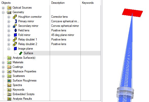
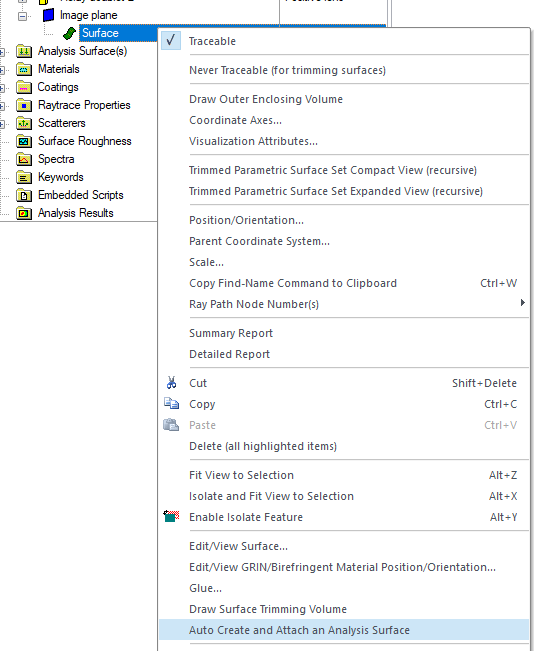
Method 3: Auto-Creation from Object Tree Right mouse click on a surface node in the object tree and choose the option, “Auto Create and Attach Analysis Surface”. We will refer to the surface node that was selected as the target surface.
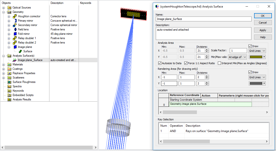
A new Analysis Surface will be added to the Analysis Surface(s) folder whose starting coordinate system is set to match the target surface and whose Ray Selection criteria is set to include only rays that are on the target surface. The Analysis Surface dimensions are set to use the Autosize to Data option (i.e. the width of the analysis surface is determined at the time of analysis by evaluating the maximum spatial extents of the ray intercepts on the target surface).
The name of the Analysis Surface is constructed from the hierarchical name of the target surface by dropping the reference to the Geometry folder and replacing the “.” characters with “_”. If, for example, the full hierarchical name of the target surface is “Geometry.Subassembly 1.Element.Surface 1”, the corresponding name of the auto created analysis surface would be, “Subassembly 1_Element_Surface 1”.
The graphics below show the auto creation process applied to a surface of interest where rays are known to exist at the conclusion of a raytrace.
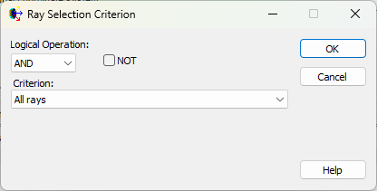
Example 2 – Accessing the Ray Selection Criterion Dialog Open the analysis plane dialog by double clicking an analysis plane on the object tree. The Ray Selection spreadsheet is found at the bottom of this dialog with the following table columns:
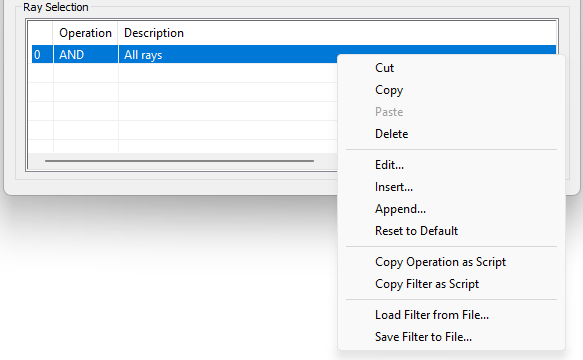
Right mouse click in the spreadsheet area to open a list of menu options as shown below.
The ‘Cut,’ ‘Copy,’‘Paste,’and ‘Delete’ options operate accordingly on the selected row. The ‘Edit…’, ‘Insert…’, and ‘Append…’ options open the Ray Selection Criterion dialog and allow modification of the current ray filter list:
The 'Copy Operation / Filter as Script' options copy either the row or the entire filter to script commands (to be pasted into the script editor). The 'Load/Save Filter' options allow the save/load of FRED Filter Collection (.ffc) files.
Analysis Surface(s) Tree Folder
|
|||||||||||||||||||||||||||||||||||||||||||||||||||||||||||||||||||||||||||||||||||||||||||||||||||||||