This command generates a ray position spot diagram using rays filtered by the selected analysis plane. The axes of the position spot diagram represent the local X and Y axes of the analysis plane.
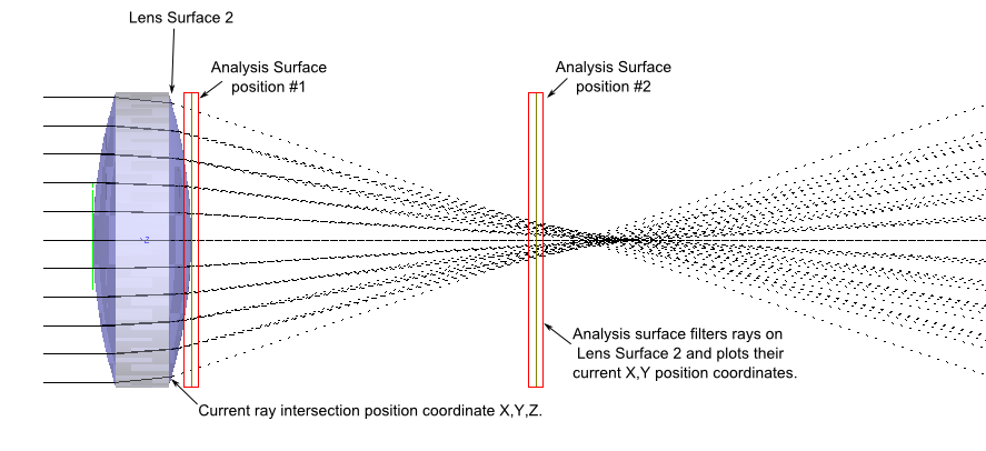
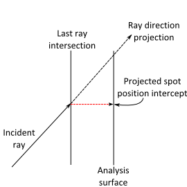
The positions of the rays included in the spot diagram are the X and Y coordinates of each ray on the surface with which they are currently associated. For example, consider the singlet system shown below in which an analysis surface is filtering rays on the back surface of a lens element. A positions spot diagram analysis at either position #1 or position #2 would show the same result, though the free space propagation clearly shows that the beam footprint should be smaller near the lens focus. The reason for this is that the rays being included in the result are associated with Lens Surface 2, and so their X, Y position coordinates are fixed there in FRED's internal ray structure until they intersect another surface in a raytrace.
This command can be accessed in the following ways: •Menu > Analyses > Positions Spot Diagram •Ctrl + F9 •Toolbar button:
Spot diagram between two elements The simplest method for analyzing the beam footprint between two optical elements is to use an intermediate transmitting plane and analysis surface in conjunction with FRED's advanced raytrace utility. Consider the following layout in which the goal is to observe the beam footprint between the two lens elements. The intermediate plane is defined using materials Air/Air, a 100% transmitting coating, and a transmit specular raytrace control so that the rays are undeviated in the airspace between the two lens elements. The intermediate plane allows use of the advanced raytrace utility so that rays can be temporarily halted at that position for an analysis and then be continued on after the analysis is complete.
Step 1: Use the advanced raytrace utility to trace rays up to the intermediate plane.
Step 2: Perform a positions spot diagram analysis using an analysis surface attached to the intermediate plane.
Step 3: Use the advanced raytrace utility to continue tracing rays through the system.
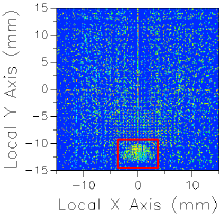
Image Artifact Diagnostic Tool If a raytrace has been performed using the Advanced Raytrace option with ray paths enabled, contributing raypath information for a particular region of interest can be reported directly from the chart view for an incoherent spatial analysis or analyses using a Directional Analysis Entity. This feature can be executed by holding down the ALT keyboard button while using the mouse to select a region of the main chart view (turn of "perspective view" using the right mouse button menu option). This procedure is outlined in the following example:
The image artifact diagnostic tool will print the following information to the output window: •Analysis surface used •Selected region x-min, x-max, y-min and y-max •Path number, path power and ray count for each contributing ray path (up to the first 30 paths, sorted by power) •Remaining path count and total power for paths not listed in the output window
Chart crosshairs are available by holding the left mouse button down inside the plot. The plot value under the cursor is reported at the bottom of the chart in both direction cosines and angles (both relative to the local analysis plane X and Y axes).
Right mouse clicking in the chart view brings up a list menu that contains the item "Move Profile Lines To". The options on the sub-menu list can be used to precisely and rapidly locate the crosshairs at common positions of interest.
|
||||||||||||||||||||||||||||||||||||||||||||||||||
.png)
.png)