This Advanced Tutorial contains some of FRED's more advanced features including 1) calculation of the Point Spread Function (PSF) using the Irradiance Spread function, 2) calculation of the Optical Transfer Function (OTF) from the PSF, and 3) inclusion of scatter typical to polished surfaces.  The system units for this tutorial are centimeters.

Note: The videos included in this tutorial are hosted by YouTube and an internet connection is required to view them.  Controls embedded into the video player will allow you to view the videos in full screen and/or change the video resolution.

Point Spread Function

The first task of this Advanced Tutorial will be to compute the Point Spread Function (PSF) for our Single Lens Reflex Camera. The PSF arises from diffraction effects which are intimately connected to the wave nature of light. While FRED is strictly a raytracing application, it has the ability to model diffractive effects by means of a Complex Raytracing algorithm, the concepts of which have been employed in other software for the last three decades. This algorithm treats each ray in the source grid as a Gaussian beamlet whose phase and amplitude can be calculated at any point along the ray trajectory. These beamlets display the properties of Gaussian beams in that they have a beam waist radius ω₀ and a divergence half-angle θ which, in the far field, is dictated solely by ω₀ and the wavelength λ. For a more detailed discussion of these Gaussian beamlets, the reader is referred to the Intermediate section of the Laser Illuminator Tutorial and to the Help article Introduction to Coherent Sources.

One simple change need be made to our source definition in order to calculate the PSF. Open the dialog for "Source 1" and navigate to the Coherence Tab. Note that the default setting for all sources is "Not Coherent" meaning that all rays are treated as incoherent and therefore not capable of displaying coherent effects such as diffraction or interference. Select the option "Coherent" as shown in Figure 3-1. Navigate to the Positions/Directions Tab and enable only the 0° field angle and press the Apply button.

Figure 3-1. Detailed Source Coherence Tab

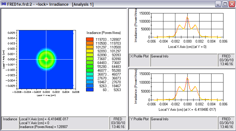
For convenience, add a second Analysis Surface setting the number of Divisions to 101x101. Leave the remaining settings in their default state. Drag-and-drop this Analysis Surface from the Analysis Surface(s) folder onto the image plane surface, "Geometry.camera.Surface 8.Surf 8", in the Geometry folder. Open the Advanced Raytrace dialog, select the option Sequential using a user-defined path under Raytrace Method and choose the DefaultSequential path. Trace the rays by pressing the Apply/Trace button (recall that the Apply button leaves the dialog box open for subsequent use) then perform an irradiance calculation using the newly added Analysis Surface. Figure 3-2 shows the resulting calculation.

Figure 3-2. Irradiance for 0° field angle at nominal image position.

Since the lens has an f-number of approximately 5, the first Airy ring is expected at 1.22λƒ# ~ 3.3 μm. The fact that the profile in Figure 3-2 seems to disagree with this calculation leads toward a conclusion that the lens may not be properly focused. FRED's Best Geometric Focus feature can be used as a quick check. Initiate a best focus calculation by one of the following methods [Note that it is not necessary to re-trace the rays.]:

1.From the Main Menu, Analyses>Best Geometric Focus

2.Keystroke Shft+F9

3.Analysis Toolbar button

The default dialog box for Best Geometric Focus is shown in Figure 3-3a. Note that the calculation can be performed in any coordinate system and has Ray Selection Criteria similar to the Analysis Surface. To determine how far the image plane is from the best focus position, set the Coordinate System to that of Surface 8. Also, only rays on the image plane are to be considered in the calculation. Thus, the dialog should be edited to reflect these settings as shown in Figure 3-3b. Press the Apply or OK button and the results of the calculation are printed to the Output Window as shown in Figure 3-4. We find that the image plane is shifted 0.0309 cm from its optimum position.

Figure 3-3. Best Geometric Focus dialog. (Top) Default and (Bottom) configured to compute image plane shift.

Figure 3-4. Best Geometric Focus output using settings in 3-3.

This focus shift can be dealt with in one of two ways: 1) Physically shift the image plane by the given amount, or 2) apply this shift to the Analysis Surface only. In the first case, the model configuration is being changed so the rays must be re-traced before another calculation is made. In the second case, no re-trace is required since only the Analysis Surface is being edited (Analysis Surfaces only post-process ray data, and do not affect the rays during the trace). Applying the shift in this manner causes FRED to internally propagate the relevant rays along their current trajectories to the Analysis Surface plane before carrying out the calculation. [Note: This is a free-space propagation and cannot take into account optical elements either up-stream or down-stream from the Analysis Surface.] This capability has wide-reaching consequences allowing the irradiance to be calculated at various positions between optical elements.

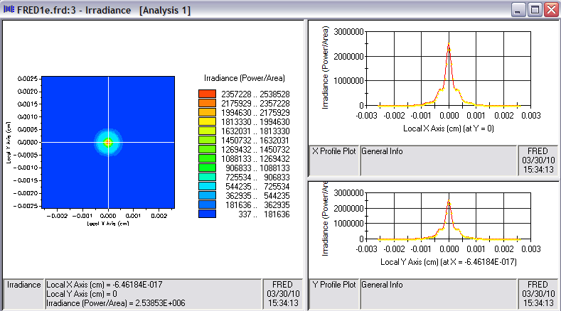
For this exercise, we choose the second option and apply the shift only to the Analysis Surface as shown in Figure 3-5. The resulting irradiance calculation shown in Figure 3-6 is more compact (note XY scale reduced by 2x) and has a higher peak value (20x increase) confirming the earlier suspicion that the lens was out of focus.

Figure 3-5. Analysis Surface with focus shift added.

Figure 3-6. Irradiance at image plane after adjustment for best focus.

Modulation Transfer Function (MTF)

The Modulation Transfer Function (MTF) can be computed directly from the PSF by normalizing its Fourier Transform. This definition is particularly convenient in evaluating system performance in the presence of stray light effects such as ghosting and scatter.

To perform a Fourier Transform operation without cell padding,  2ⁿ pixels should be defined in the Analysis Surface definition. The width of the Analysis Surface must also be set accordingly to accommodate the cutoff frequency of the lens, namely

          w = (N/4) ∙ λƒ#

where w is the Analysis Surface half-width, N (=2ⁿ) is the number of pixels across the Analysis Surface, λ is the wavelength and ƒ# is the f-number. From Figure 3-4, we have ƒ#=5.1 and a center wavelength of 0.54 μm such that the cutoff frequency v_c=1/(λƒ#)=360 lpmm. To that end, we select N=128 which yields w=0.0088128 cm. The properly configured Analysis Surface dialog is shown in Figure 3-7.

Figure 3-7. Modifications to Analysis Surface for MTF calculation.

Recall that editing of the Analysis Surface parameters does not require rays be re-traced. Therefore, a re-calculation with modified Analysis Surface settings completes the initial step of the MTF calculation. The Fourier Transform and the Normalization operations are available directly from the Chart drop-down menu. The movie clip in Figure 3-8 to shows the complete MTF calculation steps, starting from the chart window of an Irradiance calculation performed using the newly configured Analysis Surface.

Figure 3-8. Calculation of MTF from Irradiance (Video).

Surface Scattering and Associated Tools

One of FRED's greatest strengths lies in its capabilities related to stray light. In the Intermediate section, we examined ghost paths which are a significant aspect of stray light. An equally important but distinctly different aspect of stray light is scattering. While a discussion of scatter model types and the related physics is beyond the scope of this tutorial, this section focuses on the usage of tools in FRED associated with scatter calculations. Of significant importance to the overall efficiency of raytracing in the presence of scatter is the "Scatter Direction Region of Interest" which allows scattered rays to be generated only in specific directions. Clearly, there are cases such as integrating spheres and backlight displays where scattered rays must be generated in all possible directions. However, there are also classes of scatter problems where scattering rays in all directions is highly inefficient. One of these cases in particular is that of an imaging system where only rays which reach the image plane are of concern.

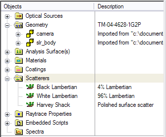
The objective of this section will be to assign a scatter model and demonstrate the methodology involved in set up of a "Scatter Direction Region of Interest" for the case of an imaging system, namely the camera lens. We begin by identifying an appropriate scatter model. The Scatterers folder in the Object Tree contains three default scatter models that accompany all FRED documents as shown in Figure 3-9. The Harvey Shack model is included as representative of scatter from polished surfaces such as lenses and mirrors. Details on this scatter model (and others) can be found elsewhere in the Help. For the purposes of this tutorial, we will make use of this default model.

Figure 3-9. Scatter model folder with default entries.

Open the dialog for the Harvey Shack model by double-clicking on its entry in the Scatterers folder. We will accept the default values for b0, L & S. Note the Additional data options Apply on Reflection, Apply on Transmission are both checked as defaults. Note that the equation for the Harvey Shack Bi-Directional Scatter Distribution Function (BSDF) is displayed in the dialog. Since this particular exercise will deal only with scatter in transmission, i.e., scatter towards the image plane, uncheck the option Apply on Reflection. The option Halt Incident Ray is unchecked and will be left in that state since the surface is a highly specular surface. The intent then is to generate scattered rays in addition to the specular component. Under this condition, FRED will subtract the Total Integrated Scatter (TIS) power from the incident ray before allowing the specular component(s) to proceed. Accept the changes as shown in Figure 3-10 by pressing the OK button.

Figure 3-10. Harvey Shack scatter model dialog.

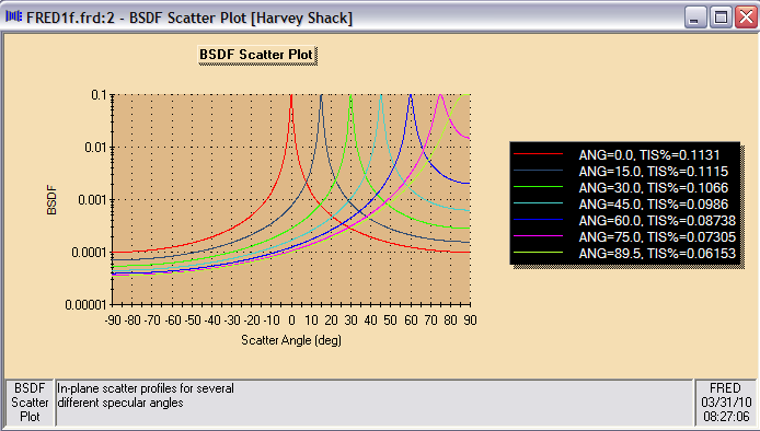
A convenient and helpful feature in FRED's GUI interface is the ability to generate plots for any Scatterer, Coating or Material.  Highlight the Harvey Shack entry in the Scatterers folder, right-click and choose the option Plot 2D (Angle) near the bottom of the pop-up menu. The plot shown in Figure 3-11 will promptly appear. This log-plot is of the BSDF versus scatter angle for selected angles of incidence. Note also the TIS values for these angles are tabulated in the legend on the right of the plot. For the particular parameters of this Harvey Shack model, scatter removes only a fraction of a percent of the total flux from an incident ray.

Figure 3-11. BSDF plot for Harvey Shack scatter model.

The next task is to assign this scatter model to the lens surfaces in our model. Therefore, we return to the Edit/View All Surfaces dialog first introduced in the "Multi-Surface Editing of Optical Property Assignments" section of the Single Lens Reflex Camera Intermediate tutorial (Figure 2-19). Open this dialog and highlight the six lens surfaces by depressing the Ctrl key and clicking on the appropriate rows. Under Modify All Highlighted Spreadsheet Rows, select "Scatter 1" from the left-most drop-down list and choose Harvey Shack from the drop-down list on the right. Press the "Replace" button, noting that this scatter model has been assigned to the selected surfaces. Since scatter is the primary focus of this section, also "Replace" the Allow All Raytrace Property with Transmit Specular in the same manner. Note that the "Replace" button serves only to edit the spreadsheet but does not effect these changes to the model. The "Apply" or "OK" button must be pressed in order to commit these changes to the model. These changes will allow the reader to return to the simple method of raytracing using the Trace and Render Toolbar button without generating multiple reflections. The movie clip in Figure 3-12 shows these edits carried out.

Figure 3-12. Using the Edit/View Multiple Surfaces dialog to assign scatter models to lens surfaces (Video).

Having assigned the Harvey Shack model to our lens surfaces, open the dialog box for the second surface of the third lens "Geometry.camera.Lens 6-7.Surface 7" and navigate to its Scatter Tab as shown in Figure 3-13. Note the presence of two general sections in this dialog tab, Scatter and Scatter Direction Region of Interest. The Scatter section lists the Available Scatter Properties containing scatter models from the Scatterer folder on the right-hand side. New scatter models can be created (Create New..) or existing scatter models can be edited (Edit/View) using the buttons provided. The Assigned Scatter Properties box lists all scatter models currently assigned to the surface. [More than one scatter model can be assigned to a given surface.] Note the check box next to the Harvey Shack model which allows the model to be enabled or disabled.

Figure 3-13. Scatter Tab for "Lens 6-7.Surface 7".

Next we turn our attention to the bottom portion of the dialog, Scatter Direction Region(s) of Interest. All surfaces in FRED are assigned a Default "Scatter Direction Region of Interest" at the time of creation. This Default entry scatters rays into 2π steradians about the surface normal. Double-click on this entry or highlight it and press the Edit/View button to open its dialog box as shown in Figure 3-14. Note the dialog box title. The terms "Scatter Direction Region of Interest" and "Importance Sampling Specification" are used interchangeably.

Figure 3-14. Dialog box for Importance Sampling Specification

There are six types of Importance Sampling Specifications. Detailed descriptions of these are provided in Scatter Properties Help topic. The Other Data section provides additional parameters for controlling the functionality of this feature and are also discussed in the Help documentation. We accept the default settings for these parameters in this demonstration.

In many cases, the most efficient type of importance sampling in the context of a lens system is Scatter rays through a closed curve where the closed curve is a rectangle representative of the rectangular image plane. From the perspective of each lens surface, the image plane has a different apparent size and location influenced by the intervening optical surfaces between it and the image plane. To illustrate this point, consider the image plane as viewed from the back surface of the last lens. Here, the image plane obviously appears with its actual physical size and location since no other optical elements are involved. Thus, the closed curve used as an Importance Sampling Specification would be a rectangle the size of the image plane and located at the image plane. Consider now the appearance of the image plane when viewed from the front surface of the last lens. Its apparent size and position are now influenced by the shape of the lens second surface and lens thickness as well the material refractive index. This principle applies to each lens surface. In general, the image plane will have a different apparent size and location associated with each lens surface.

First, let's add the Importance Sample for the back surface of the last lens since it is a simple matter of creating a rectangular closed curve with the same dimensions and located at the image plane. Add a new Custom Element under the camera subassembly. A Custom Element can be added by one of the following methods:

1.From the Main Menu, Create>New Custom Element

2.Keystroke Ctrl+Alt+E

3.Create Toolbar button

4.Right-click on the Subassembly and select the option Create New Custom Element

Name this Custom Element "Importance Sample Curves". With the new Custom Element still highlighted in the Object Tree, create a new curve by one of the following methods:

1.From the Main Menu, Create>New Curve

2.Keystroke Ctrl+Alt+V

3.Create Toolbar button

4.Right-click on the Custom Element and select the option Create New Curve

This action opens a New Curve dialog box. Select the curve type Segmented (points connected by line segments) from the drop-down Type list then right-click in the dialog table to expose another drop-down menu. From these choices, select the option Generate Points. This selection opens the Segmented Curve Generation dialog. In the Dimensions and Sampling section, enter a four (4) sided curve with X semi-width 2 and Y semi-width 1.5 per the image plane semi-apertures. Select the option Top edge parallel to x-axis in the Orientation section and Circumscribe under the Type section. Press the OK button and FRED automatically fills in the Segmented curve XYZ point entries. Navigate to the Location/Orientation Tab and set the Reference Coordinate System to .camera.Surface 8, the Custom Element containing the image plane.  The steps described above are demonstrated in the movie clip of Figure 3-15.

Figure 3-15. Adding a new Custom Element and an Importance Sample curve (Video).

Open the surface dialog for "Geometry.camera.Lens 6-7.Surface 7". Navigate to its Scatter Tab and double-click on the Default "Scatter Direction Region of Interest" entry to open its dialog. Select the type Scatter rays through a closed curve then select the newly created curve ".camera.Importance Sample Curves.Curve 1". Rename this "Importance Sampling Specification" to "Edge for Lens6-7.Surface 7" as shown in Figure 3-16. Press the OK button on this dialog to accept these changes then press the OK button on the Surface dialog box finalize the assignment.

Figure 3-16. Importance Sampling Specification for Lens 6-7.Surface 7.

It is highly recommended that each new Importance Sampling assignment be tested. FRED offers a feature designed specifically for this purpose. The Analyze Scatter Importance Sampling feature is found on the Tools Main Menu. To test the Importance Sample created above, select the image plane surface (Geometry.camera.Surface 8.Surf 8) as the "Detector" Surface to Scatter Toward, check the Test box for Lens 6-7.Surface 7, enter 1000 in the # Rays column then check both boxes at the bottom right of the dialog to Print efficiency results to the text window and Draw the rays used to compute the efficiency as shown in Figure 3-17. Press the Analyze button and examine the raytrace shown in the 3D View and the Output Window as shown in Figure 3-18.

Figure 3-17. Importance Sampling Analysis Tool. Testing of scatter from Lens 6-7.Surface 7.

Figure 3-18. Results of Importance Sampling Efficiency test.

Two observations are worth noting from Figure 3-18. First, the image plane is fully flooded with rays indicating that the closed curve has been correctly positioned and sized. No rays are missing the image plane. Secondly, the Output Window shows an efficiency of ~94%. This value indicates that, in this case, the remaining 6% of the rays intersected the lens housing. This can be verified by re-running the test after making the lens housing and camera body Untraceable as shown in Figure 3-19.

Figure 3-19. Analyze Importance Sampling test re-run with lens housing and camera body Untraceable.

We now continue with the more complicated task of assigning Importance Samples to the remaining lens surfaces. This process requires using the eight (8) steps outlined below. In summary, these steps are designed to identify the apparent size and location of the image plane as viewed from any given surface in the imaging system. Note:  This recipe assumes the system is in-line and aligned along the z-axis. It will be left as an exercise for the user to generalize this method to folded optical systems.

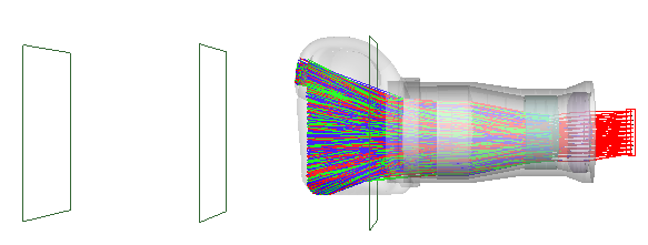
Figure 3-20 shows a raytrace where Scatter Direction Regions of Interest have been set for all lens surfaces according to the steps shown above. This task has been performed using a script based upon these steps and is included as part of the example file tutorialSLRAdvanced.frd located in the <install dir>\Resources\Samples\Tutorials & Examples\ directory. A Ray Summary will show that over 80% of the total rays traced reach the image plane. This percentage drops only slightly to 77% even when the lens is flooded over its entire entrance aperture.  The fact that the efficiency is not 100% is indicative of the fact that few if any optical systems are well-corrected from the point of view of each intermediate surface.

Figure 3-20. System illuminated at 0°, 5° & 10° with importance samples set for each lens surface.