In this Intermediate Level Tutorial, complexity is increased by 1) importing a lens prescription and CAD geometry, 2) creating a Detailed Source with multiple field angles, 3) adding coatings and custom materials, 4) applying optical properties with the multi-surface edit feature, 5) carrying out a basic ghosting analysis using Raypath features, and 6) using supplemental plotting & visualization features. The system units for this tutorial are centimeters.
Note: The videos included in this tutorial are hosted by YouTube and an internet connection is required to view them. Controls embedded into the video player will allow you to view the videos in full screen and/or change the video resolution.
Importing a Lens Prescription and Camera Housing
Modern optical engineers are often faced with a requirement to integrate existing lens systems and opto-mechanical assemblies designed using other software applications. In particular, lens systems are generally designed, optimized and toleranced in one of several lens design programs specially suited for this task. Computer Aided Design (CAD) programs are routinely used in industry to design mechanical hardware as well as some types of optical elements such as reflectors and lightpipes. FRED provides import routines capable of bringing these branches of optical engineering disciplines together in a single environment.
FRED provides an import routine for reading lens prescriptions from the most widely used lens design programs in the industry: CodeV, Zemax & OSLO. Table 2-1. below lists the recognized file extensions for these programs.
Table 2-1. Lens Import File Extentions
*FRED does not read Zemax non-sequential data
Care must be exercised when importing lens prescriptions with regard to glass materials and catalogs. FRED attempts to match common glass names to entries in its catalogs or uses private catalog data embedded in the prescription files for CodeV and OSLO. Zemax files carry a list of catalog names from which index data is retrieved. Thus, any catalogs referenced within Zemax prescriptions must reside in the same directory as the *.zmx file being imported. For more information, see the Help topic Lens Import.
This tutorial begins by importing a Zemax file from the Tutorial directory included with your FRED installation. For the purposes of this tutorial, we start with no FRED document open although it is possible to import into existing FRED documents. The lens import feature is accessed from the Main Menu File>Import>Import Optical. Navigate to the the FRED installation directory:
C:\Program Files\Photon Engineering\FRED X.xx.x\Resources\Samples\Tutorials & Examples
Select the file "camera.ZMX". All files to be imported in this section are found in the directory indicated above.
Figure 2-1. Lens Import Dialog
Figure 2-1 above shows the Lens Import dialog once the file has been selected. The option Add Analysis Surface to image surface has been checked in the Import Options. Otherwise the dialog has its default settings. For more details on importing lenses, see the Help topic Lens Import. Select the "Create" button then "Dismiss" the dialog. As in Figure 2-2 below, your 3D View should now show the camera lens. Note also the entries in the Geometry, Analysis Surface(s), and Material folders. Surface 1 is the lens stop and surface 8 is the image plane. All six lens surfaces have even asphere definitions. Note also that the system units are now in centimeters as indicated in the Summary box in Figure 2-1.
Figure 2-2. Imported lens "camera.ZMX"
Importing a lens from a prescription file (*.zmx, *.seq, *.len) causes FRED to "learn" both the default sequential and reverse sequential paths as part of the import operation. Open the list of User-defined paths using one of the following methods:
1.From the Main Menu, Raytrace>User-defined Ray Paths 2.Keystroke Ctrl+Shft+U 3.Raytrace Toolbar button
From the drop-down Selected Path list, select DefaultSequential as shown in Figure 2-3. Note that the Stop Surface is at the top of the list. Since the source added in the next major section will be co-located with the Stop, this entry should either be removed from the list or designated as non-sequential. Check the box in the "Non Seq" column of the first row and press the OK button. This saves this change to the DefaultSequential path. We will use this path later on in this section.
Figure 2-3. User-defined Ray Paths dialog with Default Sequential path selected.
Note in Figure 2-2 that the image plane surface has entered the model as a circular plane. Expand the Custom Element Surface 8 and open the dialog for Surf 8 by double-clicking on its icon in the Tree folder. Navigate to the Aperture Tab and set the X & Y semi-aperture of the Trimming Volume Outer Boundary to 2 cm and 1.5 cm, respectively. Select the Shape type "Box" to create a rectangular image plane. Figure 2-4 shows the Aperture Tab with the new size and shape.
Figure 2-4. Image plane dialog box. Settings for Trimming Volume Outer Boundary.
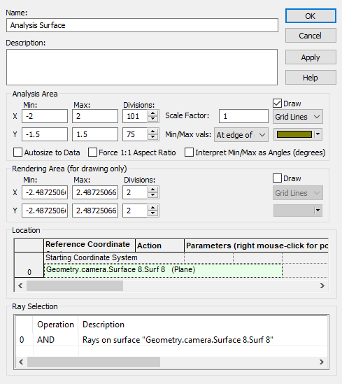
Open the Analysis Surface dialog by double-clicking on its entry in the Tree folder and set its X & Y Min/Max limits to match the image plane dimensions. Also set the number of Divisions to 101x75 in proportion to the rectangular area as shown in Figure 2-5. Note that odd numbers for Divisions leads to a pixel centered on the local origin of the Analysis Surface.
Figure 2-5. Analysis Surface dialog. Analysis Area sized to image plane and increased resolution.
Now zoom in on the first camera lens (purple) by left-clicking in the 3D View then hovering the cursor over the lens and using the mouse roller. Note the ragged nature of the lens surfaces. These are OpenGL artifacts associated with tessellation that often accompany complex surfaces. Right-click on the camera subassembly in the Tree and select the option Visualization Attributes. Settings in this dialog will apply to all entities within the subassembly. Go to the lower left-hand corner of the dialog and check the option Reset Tessellation and click "Apply". A second application is necessary in this case to produce smooth visualization of the aspheric surfaces. [Care should be taken not to over tessellate as this will cause the 3D View to be less responsive to rotation, translation, zooming & updating. Note, however, that the level of tessellation has no effect on raytrace accuracy or fidelity since all surfaces are internally traced as mathematical representations.]
Figure 2-6. Re-tessellating the camera lens (Video).
We will now import two pieces of CAD geometry; a simple lens housing designed for the camera lens and a modified SLR camera body. Import the lens housing from the Main Menu, File>Import>Import CAD (or keystroke Ctrl+Shft+J) and select the STEP file lens.housing.1.stp as shown in Figure 2-7 below insuring that the Destination option Import into Current Document is selected. Note the Surface Drawing Mode default setting is Wire frame (fast) and is recommended initially especially in the case where a large number of objects are present in your CAD geometry. Accept the default settings by pressing the "Create" button. Once the import is complete, press the "Dismiss" button to clear the dialog. For more information on import of CAD geometry, see the Help section CAD Import.
Figure 2-7. Importing the camera lens housing.
The lens housing enters the FRED document with its front face at the global origin since this position was used as the datum in the CAD program. A z-shift of 1.32 cm will be required to align the lens housing with the lens elements. For the purposes of organization and simplification, we now drag-and-drop the lens.housing.1 subassembly into the camera subassembly. It is important to note that moving the lens.housing.1 subassembly into the camera subassembly does not change the Starting Coordinate System of lens.housing.1. We therefore must re-parent the lens.housing.1 subassembly then add the z-shift.
Figure 2-8. Reparenting and shifting lens housing (Video).
The final step of geometry construction is import of the camera body from CAD. Import the file SLR_body.stp. This portion of the geometry has its origin where the film plane should be located. Therefore, we need to import and then re-position the camera lens and housing. Once the SLR body is imported, a 180° rotation about the y-axis and z-translation of the camera subassembly by 10.58 cm places all the geometry in its proper relationship. For a more pleasing appearance, and the Visualization attributes of the camera housing and SLR body have been set to Smooth Shading and partial transparency. The complete SLR camera along with these steps is now shown the movie clip Figure 2-9. The image plane has been re-sized to x=+/2cm and y=+/-1.5cm.
Figure 2-9. Rotation/shift of camera subassembly. Visualization Attributes reset (Video).
Creating a Detailed Source with Multiple Field Angles
Upon completing the import of our geometry, we now add a source with several field angles. This is easily accomplished through the Detailed Source construct. The Detailed Source offers increased flexibility for setting source characteristics beyond what is provided with the Source Primitive types. Among these are numerous grid position & direction types, various positional & directional apodization options, explicit control of polarization states and additional visualization options. A Detailed Source can be created by one of several methods:
1.From the Main Menu, Create>Detailed Source 2.Keystroke Ctrl+Alt+D 3.Right-click on Optical Sources folder in Tree and select Create New Detailed Optical Source 4.Create Toolbar button
Figure 2-10 shows the default dialog for a Detailed Source. Note the eight tabs where various source properties are managed. In this section, we will use three of these tabs; the Positions/Directions Tab to set up the grid dimensions, number of rays and their directions, the Location/Orientation Tab to re-parent and locate the source, and the Wavelength Tab to create multiple wavelengths.
Figure 2-10. Detailed Source default dialog.
Moving first to the Positions/Directions Tab as shown in Figure 2-11, set the ray position as a Grid Plane type with 31x31 rays across the elliptical (circular) aperture of semi-width 0.7857 cm (see the Aperture Tab of Surface 1.Surf 1, the Stop surface). For ray Directions, we select the Multiple Source angles (plane waves) type from the drop-down list. This option allow multiple source angles to be defined in terms of angle with respect to the source local x- and y-axis. For this tutorial, we choose y-angles of 0°, 5° & 10°. Note that each angle row has a check box allowing specific angles to be toggled on or off.
Figure 2-11. Detailed Source Positions/Directions Tab.
Next, the source is properly positioned with respect to the lens by simply setting the source to be in the coordinate system of the Stop surface on the Location/Orientation Tab as shown in Figure 2-12. Note that the additional Z shift of -0.001 is to break the coincidence between the source node, where the rays originate from, and the Stop, Surface 1. The offset, which can be made almost arbitrarily small, guarantees that there is no ambiguity about whether or not the rays intersect Surface 1 when they leave the source. When there is coincidence, the limits of numeric precision will dictate whether or not the rays intersect Surface 1.
Figure 2-12. Location/Orientation Tab parenting the source to Stop surface.
Finally, we move to the Wavelength Tab and add three wavelengths by selecting the option Set Standard Bitmap Wavelengths (see Figure 1-13). Once these wavelengths are tabulated in the list, set the Draw colors of these wavelengths using the option Set All Colors from Wavelengths. A short clip illustrating this process is shown in Figure 2-13.
Figure 2-13. Choose source wavelengths as RGB and set corresponding draw colors (Video).
Adding Materials and Coatings
A closer look at both the native FRED lenses created in the Basic section and the imported lenses from this section will reveal that the lens surfaces are each assigned a Transmit coating. The Transmit coating has R=0, T=1 and is one of the five default coatings appearing in every FRED document as shown in Figure 2-14 below. The Transmit coating is a convenient choice for the initial stage of analyses since it allows for transmission only, generating no reflected ray and thus requiring no splitting. In fact, the Transmit, Absorb, Reflect and Standard coatings are not strictly physical coatings since they have no angular or polarization dependence. In contrast, the Uncoated coating is a physical coating exhibiting the appropriate angular dependence and polarization-related properties representative of a bare substrate.
Figure 2-14. FRED's default coatings.
This section will highlight the methodology involved in adding new materials and coatings to your FRED model. For the purposes of this exercise, we will make two simple coating types; a Sampled Coating and a Quarter-wave Single Layer coating. These and other coating types can be created by one of several methods:
1.From the Main Menu, Create>New Coating 2.Keystroke Ctrl+Alt+C 3.Right-click on the Coatings Folder in the Tree and select Create a New Coating 4.Create Toolbar button
The Sampled Coating is an idealized coating in which the reflectance and transmittance (and fixed phase shifts associated with each) at any number of wavelengths can be entered in table format. If only one wavelength is entered, then the given reflectance and transmittance are applied to all wavelengths. Figure 2-15 shown below illustrates the definition of a coating with 1% reflectance and 99% transmittance at the default wavelength. Once the information is added and the OK button is selected, this coating appears in the Coatings folder and can be used on any surface in the FRED model. Note that this coating has no polarization dependence.
Figure 2-15. Ideal Low Reflectance Coating (Sampled type)
Properties of the Quarter-wave Single Layer coating type are defined by the standard amplitude and phase equations associated with thin films. As such, this coating type requires the definition of a layer material prior to creating the coating. For this exercise, we will create a simple model of Magnesium Fluoride (MgF2) with refractive index 1.38 at the default wavelength 0.58756mm as shown in Figure 2-16. New materials are created by one of several methods:
1.From the Main Menu, Create>New Material 2.Keystroke Ctrl+Alt+T 3.Right-click on the Materials Folder in the Tree and select Create a New Material 4.Create Toolbar button
Figure 2-16. User-defined material MgF2.
With the material MgF2 added to the Material folder, create a new coating of type Quarter-wave Single Layer with this material. The movie clip below in Figure 2-17 shows the process of creating this coating type.
Figure 2-17. Creating a Quarter-wave layer coating using MgF2 (Video).
It is appropriate here to point out the distinction between two apparently related property assignments on each surface in any model; the Coatings and the Raytrace Properties. Coatings determines how power is allocated to reflected and transmitted rays when a ray encounters an interface and splits. In contrast, the Raytrace Properties determines whether the reflected or transmitted ray or both are to be traced. The names given these four default properties as shown in Figure 2-18 are self-evident; Halt All allows neither a reflected or transmitted specular ray to be created, Transmit Specular allows only the transmitted ray, Reflect Specular allows only the reflected ray and Allow All allows both a transmitted and reflected ray (if allowed by the coating properties). Numerous other attributes are controlled by the Raytrace Properties but we concentrate here only on the specular aspect. In the subsequent section on ghosting, this topic will be revisited to introduce one other important aspect integral to such an analysis.
Figure 2-18. Default Raytrace Properties
Multi-Surface Editing of Optical Property Assignments
In order to proceed with the ghosting analysis in the next section, the lenses must have Coating and Raytrace Properties that allow for both a transmitted and reflected ray at each surface. The low reflectance coating QW MgF2 created in the previous section now needs to be applied to each of the lens surfaces. It will also be necessary to change the Raytrace Properties for these lens surfaces from the default Transmit Specular to Allow All in order to allow both reflected and transmitted rays to be generated. FRED's Edit/View Multiple Surfaces feature is designed especially for such operations. This feature relieves the user from having to open and edit the individual surface dialogs.
Access the Edit/View Multiple Surfaces feature from the Main Menu, Edit>Edit/View All Surfaces. A spreadsheet-like dialog appears with a listing by row of each surface in your model. Each row contains the Traceable flag, current Material, Coating, Raytrace Properties and Scatterer assignments for the surface. To edit specific surfaces, depress the Ctrl key and highlight the row(s) of interest then move to the Modify All Highlighted Spreadsheet Rows area to change the desired properties. Note that the Replace button replaces the properties in the spreadsheet only. Actual changes to the model are not made until either the Apply or OK button is selected. This procedure is illustrated in the movie clip of Figure 2-19.
Figure 2-19. Assignment of coating and raytrace control to multiple surfaces using Edit/View Multiple Surfaces feature (Video).
Ghosting Analysis
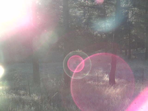
Ghosting is a specular effect resulting from multiple reflections within any system containing refractive elements. This effect is quite common in cameras manifesting itself as relatively bright spots or flares superimposed upon the image due to sources both inside and outside the field-of-view. Figure 2-20 shows an extreme case commonly encountered in amateur photography. Another form of ghost reflections come in the form of focused reflections from surfaces in lasers and beam delivery systems which can lead to surface or bulk damage of the optical components. This section of the tutorial is dedicated to introducing the tools available in FRED for diagnosis of these artifacts.
Figure 2-20. Extreme example of ghost artifacts in camera image.
As a result of the Coating and Raytrace Property assignments made in the preceding section, our camera model now has the necessary attributes to enable the formation of ghost images. First, trace the system by simply issuing a Trace and Render (
This section of the tutorial will introduce some of the features in FRED specifically designed to enable the details to be examined in a clear and informative fashion.
Figure 2-21. Camera after Trace and Render with multiple reflections.
An extremely important feature in FRED is its ability to store and access information about the myriad paths involved in the trace shown in Figure 2-21. FRED's Advanced Raytrace feature affords this capability as one of its many options. Open the Advanced Raytrace dialog by one of the following methods:
1.From the Main Menu, Raytrace>Advanced Raytrace 2.Keystroke Ctrl+Shft+A 3.Raytrace Toolbar button
While the dialog associated with the Advanced Raytrace feature shown in Figure 2-22 has numerous options, we will specifically concentrate on the two options Create/use ray history file and Determine raypaths found under the Raytrace Options section on the top right of the dialog. Note that in most cases the Draw every option under Output/Drawing Options should be unchecked to both speed up the raytrace and avoids filling the 3D View with rays which obfuscate the system geometry un-necessarily consuming video memory. Trace the rays by depressing the OK button.
Figure 2-22. Advanced Raytrace dialog configured to save path and history information.
When the raytrace is initiated with the Create/use ray history file and Determine raypaths options selected, FRED stores each intersection for each ray in a history file and groups rays into "raypaths" defined by unique sequences of surface intersections. This information is accessed through the Raytrace Paths Summaries dialog found on the Main Menu Tools>Reports>Raytrace Paths. Layout of the Raytrace Paths Summaries dialog is in spreadsheet format as shown in Figure 2-23 where each row represents a unique "path" through the system.
Figure 2-23. Raytrace Paths Summary dialog after Advanced Raytrace. Note: the paths shown may not have the same ordering for your particular computer.
Information in this table can be sorted by double-clicking on the header of any given column. Path numbers are listed in the leftmost column and total incoherent power for each path in the second column. The rightmost three columns list for each path the First Entity, Last Entity and Previous Entity, respectively. These entries tell, in order, where the path started, where the path terminated and the entity intersected prior to the path termination. The remaining columns list information relevant to the path including number of rays (Ray Count) and, of particular interest to this analysis, the number of specular reflections (Spec Refl Count).
The objective of this analysis is to examine paths which terminate on the image plane (camera.Surface 8.Surf 8). It is clear from Figure 2-23 that Path #0 contains the greatest total power (93%), terminates on the image plane and has no specular reflections. This must be the primary path from source to image plane. To confirm this assertion, highlight Path 0 in the table by clicking on that row in the leftmost path number column. Right-click on the highlighted row to expose a drop-down menu and select the option Redraw Ray History. This path is then drawn in the 3D View. The movie in Figure 2-24 shows these steps in action.
Figure 2-24. Redrawing ray history for path #0 (Video).
The next step in the analysis will be to group together all paths which terminate on the image plane. Do this by double-clicking on the Last Entity column and scrolling down until those paths appear in the table. Note there are 15 other paths in addition to Path 0 each involving two specular reflections. The movie clip in Figure 2-25 shows how to path sort and redraw of the ghost path with the most power.
Figure 2-25. Sorting on Last Entity and redrawing ghost path with most power (Video).
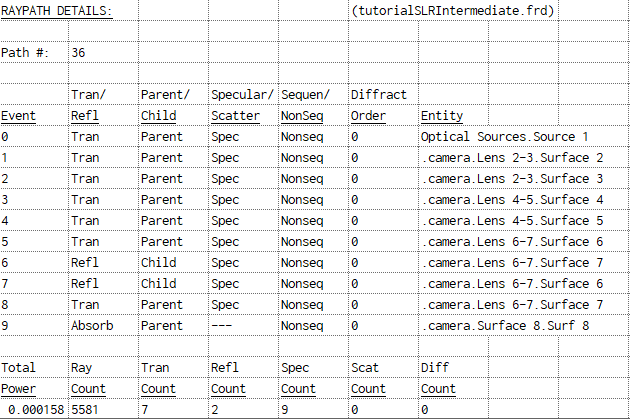
Note one of the other options on the drop-down menu is Output Path Details. This option prints a list of surface intersections for the selected path to the Output Window. Figure 2-26 shows that listing for the selected path, #36. This path involves reflections from Surface 7 then Surface 6 (Events 6 & 7) before terminating on the image plane Surf 8. This process can be repeated for any of the paths in the list.
Figure 2-26. Surface intersection listing for Path #36 from Output Path Details.
The next task of interest is the irradiance profile on the image plane. With the Analysis Surface already in place, we now run an Irradiance calculation. An Irradiance calculation is invoked using one of the following methods:
1.From the Main Menu, Analyses>Irradiance Spread Function 2.Keystroke Ctrl+F10 3.Analysis Toolbar button
The call for an Irradiance Spread Function pops a dialog as shown in Figure 2-27. This dialog allows the user to select among the available Analysis Surfaces which is to be used for the calculation. Here we have only one to choose from; Analysis Surface. However, in general, any number of Analysis Surfaces can be defined and all will be presented in this list when the Irradiance Spread Function is requested. The user must select the specific Analysis Surface to be used for the current calculation. Note also the Pre-Analysis Ray Operations options. If a raytrace has been executed prior to the Irradiance Spread Function request, then these options are unchecked. The user simply selects the OK button to proceed. On the other hand, if the Irradiance Spread Function is requested before any raytrace, these options allow for the raytrace to be executed from this dialog before the calculation proceeds.
Figure 2-27. Analysis Surface selection dialog following initiation of Irradiance Spread Function.
Figure 2-28 shows irradiance at the image plane including all 16 paths. The plot is dominated by peaks corresponding to the three field angles 0°, 5° & 10°. It is difficult to discern the effect of the ghost paths because they are spread out over the entire image plane area while the primary paths are tightly concentrated and therefore have a much higher irradiance.
Figure 2-28. Irradiance profile at image plane including all paths.
We can choose to view the irradiance plot due only to path #36 by adding an entry to the Analysis Surface Ray Selection list. Open the Analysis Surface dialog box and right-click in the Ray Selection table at the bottom. Append a new entry and set the type of the entry to Rays on the specified ray path. Enter the path number in the Value field and hit OK. There are now two Ray Specification filters; one restricting the calculation to rays on the image plane AND a second specifying rays included in path #36. The filters are applied on a ray-by-ray basis retaining rays that satisfy both criteria. Accept the changes to the Analysis Surface dialog by again hitting the OK button. Finish the process by requesting an Irradiance Spread Function calculation using the Analysis Surface. This process is show in the movie clip Figure 2-29.
Figure 2-29. Applying a Ray Specification filter (rays on path 36) to the Analysis Surface and calculating irradiance (Video).
This pattern is dominated by a bright area near the center, a weaker band across the top and what appears to be a diffuse background uniformly covering the image plane. A logical follow-on to this observation might well be "How do these features in the irradiance profile relate to the three field angles?" To answer this question, it will be necessary to trace and calculate the irradiance for the three field angles separately since the individual field angles are indistinguishable in terms of the definition of a raypath and there is no Ray Selection filter which references field angle. Dealing with this situation offers the opportunity to introduce additional functionality related to both the Raytrace Paths Summary and Advanced Raytrace.
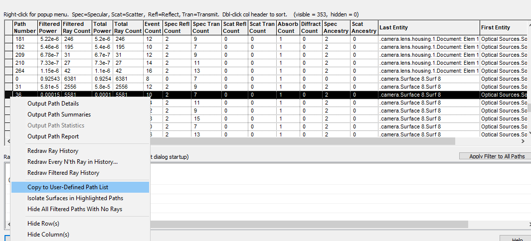
Return to the Raytrace Paths Summary dialog, highlight to row containing path #36, right-click and select the menu option Copy to User-defined Path List. as shown in Figure 2-30. This saves a copy of the sequential path associated with path #36. This specific path can now be traced as a sequential path from the Advanced Raytrace dialog.
Figure 2-30. Copying path 36 to the User-defined Path List.
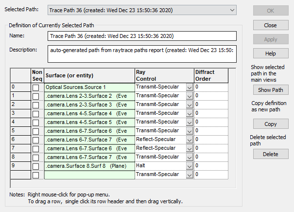
For verification purposes, return to the User-defined Ray Paths dialog as shown in Figure 2-3. The reader should now find a new entry listed as one of the choices for Selected Path. The name for this entry contains the path number along with date and time of creation. Path 36 shown in Figure 2-31 contains the list corresponding the Output Window print-out in Figure 2-26, namely, multiple reflections from Surface 6 & 7 of the third lens.
Figure 2-31. Ray Path #36 created from Raytrace Path Summaries dialog option Copy to User-defined Path List.
Next, open the Analysis Surface dialog and delete the ray path filter from the Ray Selection list leaving only the original entry Rays on surface "Geometry.Surface 8.Surf 8" (the image plane) as shown in Figure 2-32.
Figure 2-32. Analysis Surface with raypath filter removed.
Next, open the Source dialog and de-activate the 5° & 10° field angles. Finally, open the Advanced Raytrace dialog and choose the Raytrace Method Sequential using a user-defined path. Select "Trace Path 36" from the drop-down list and press the Apply button. The movie in Figure 2-33 shows this process in action.
Figure 2-33. Selecting one field angle and trace source as sequential path with Advanced Raytrace dialog (Video).
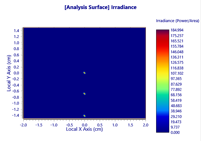
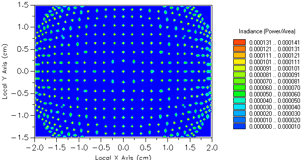
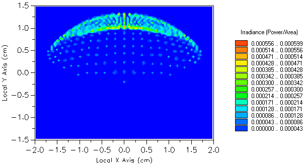
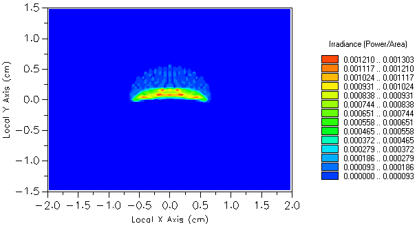
The irradiance at the image plane associated with path 36 due to the on-axis field angle can now be calculated. Repeat the process demonstrated in Figure 2-33 for the remaining field angles individually. The three irradiance profiles are shown in Figures 2-34,35 &36.
Figure 2-34. Path 36 irradiance at image plane for 0° field angle.
Figure 2-35. Path 36 irradiance at image plane for 5° field angle.
Figure 2-36. Path 36 irradiance at image plane for 10° field angle.
Figures 2-34,35 & 36 show that the ghost for the path involving multiple reflections from the third lens is most pronounced for the 10° field angle.
In the Advanced Tutorial, analysis of this lens system will be extended to include a calculation of the Point Spread Function (PSF). This will allow for a comparison of the relative magnitudes of irradiance levels associated with ghost and primary paths.
|
.png)
.png)
.png)
.png)
.png)
.png)
.png)
.png)
.png)
.png)
.png)
.png)
.png)
.png)
.png)
.png)
.png)