This Intermediate Tutorial for the Laser Illuminator introduces tools vital to coherent analyses such as the Gaussian Ray Size Spot Diagram, the Scalar Field calculation and a wavefront analysis. A configuration of the source and afocal which produces coherent ray errors will be demonstrated. The Field Resampling feature is introduced as a method of circumventing this problem.
Note: The videos included in this tutorial are hosted by YouTube and an internet connection is required to view them. Controls embedded into the video player will allow you to view the videos in full screen and/or change the video resolution.
Coherent Analyses
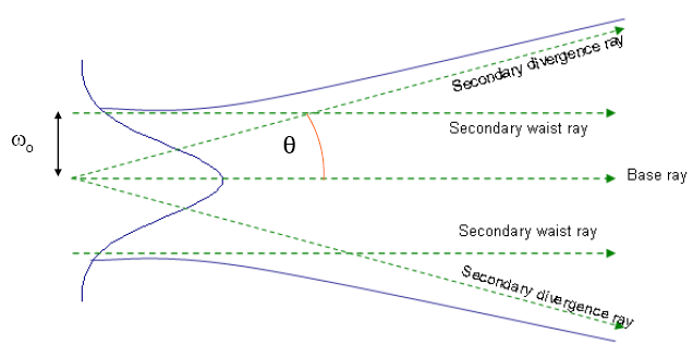
Recall from the Basic Tutorial that coherent sources consist of individual Gaussian beamlets. These beamlets are realized by tracing additional rays along with each ray in the grid. These additional rays are called "secondary rays" and are illustrated in Figure 2-1. Their genesis comes from the concept of Complex Raytracing introduced by Arnaud[1]. Each ray associated with the source grid is termed a "base" ray. There are four pairs of secondary rays termed "waist" and "divergence" rays. The "waist" ray is traced parallel to the base ray at a distance equal to the Gaussian beamlet radius ωo. The "divergence" ray begins at the position of the base ray and is traced at an angle θ defined by the Gaussian beam far-field divergence equation tan(θ)=λ/πωo where λ is the wavelength. Mathematical relationships between the base ray and its secondary rays allow the size and wavefront curvature of the beamlet to be computed at any point along the base ray trajectory. FRED keeps track of these secondary rays throughout the journey of each ray but does not draw them during the raytrace even when rays are traced using Trace and Render.
Figure 2-1. Elements of coherent rays; base ray and secondary rays.
We now introduce a tool designed to graphically display the beamlets on any selected Analysis Surface. The Gaussian Ray Size Spot Diagram draws a circular or, in general, an elliptical curve centered on each base ray of the coherent source grid representing the size and shape of the Gaussian beamlets. The Gaussian Ray Size Spot Diagram can be accessed by one of these methods:
1.From the Main Menu, Analyses>Gaussian Ray Size Spot Diagram 2.Keystroke Ctrl+Shft+G 3.Analysis Toolbar button
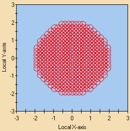
To illustrate its functionality, return to the document created in the Basic Tutorial. Use the function Raytrace>Create All Sources to generate the source rays at the source position. Invoke the Gaussian Ray Size Spot Diagram using the Analysis Surface Irradiance at laser source. Note as in Figure 2-1 the presence of overlapping circles centered on the individual rays in the grid. These circles represent the waist of each Gaussian beamlet. Recall that the size of the individual Gaussian beamlets is dictated by the spacing between rays in the grid. An additional multiplier of 1.5 termed the overlap factor is applied to the size of each beamlet for all coherent sources. This overlap factor ensures that the coherent summation of the individual beamlets produces a smooth amplitude profile. More information concerning these Gaussian beamlets can be found on the Help page Coherent Source Introduction and will be discussed in more detail later in this tutorial.
Figure 2-2. Gaussian Ray Size Spot Diagram for source as defined in Figure 1-5.
Next, trace the source rays through the afocal and again calculate the Gaussian Ray Size Spot Diagram this time using the Analysis Surface Output Beam. Figure 2-3 shows the beamlets after having passed through the optical elements. We note no qualitative difference between Figures 2-2 & 2-3 other than the fact that the individual beamlets have grown in size as should be expected.
Figure 2-3. Gaussian Ray Spot Diagram after passage through afocal optics.
The next step of our analysis will make use of the Scalar Field calculation to examine both the energy distribution (irradiance) and wavefront contour at the afocal output. The Scalar Field feature provides access to the Energy (irradiance), Field Amplitude, Real & Imaginary parts, Phase and Wavefront (waves) based upon the complex components of the coherent field. Access the Scalar Field calculation using one of the following methods:
1.From the Main Menu, Analyses>Coherent Scalar Wave Field 2.Keystroke Ctrl + Shft + W 3.Analysis Toolbar button
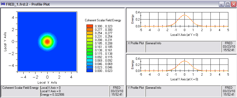
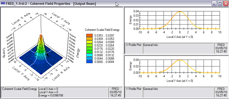
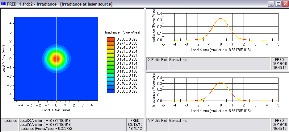
Let us now trace the source rays through the afocal telescope and make a Scalar Field calculation. The "Energy" distribution is shown below in Figure 2-4. Note that this energy distribution is identical to the irradiance distribution calculate in the Basic section as shown in Figure 1-16.
Figure 2-4. Scalar Field calculation at afocal output.
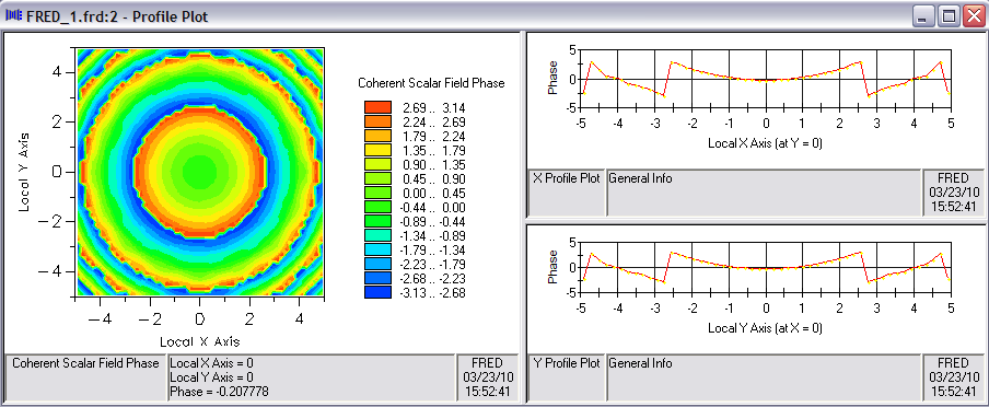
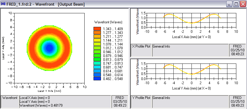
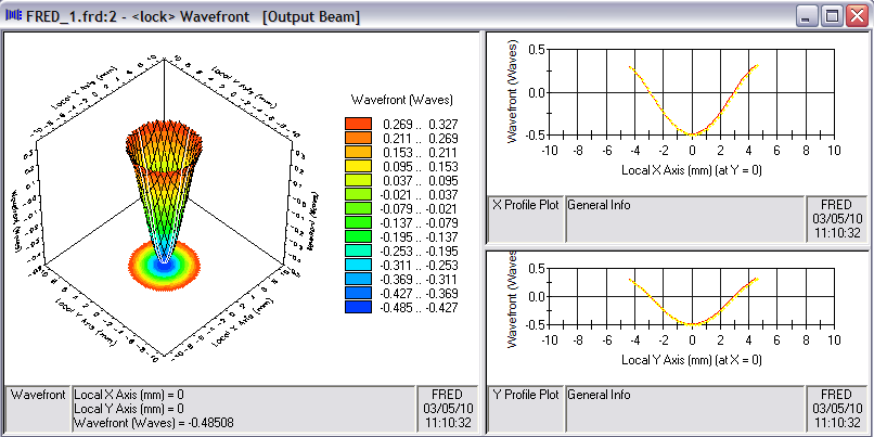
We can now view the wavefront profile of the beam shown in Figure 2-4 by right-clicking in the Chart and selecting the option Show Computed Wavefront from the popup menu. As can be seen from the chart in Figure 2-5, the beam has just more than λ/2 center-to-edge wavefront curvature.
Figure 2-5. Wavefront (in waves) of expanded HeNe laser beam at afocal output.
Alternate Configuration
Consider now the situation in which the afocal is placed a distance equal to the Rayleigh range away from the beam waist. The Rayleigh range is defined as ZR = πω02/λ which, for the initial input beam with ω0=1mm and λ=0.6328 μm, is a distance of approximately 5 meters. Apply a shift of -5 meters in the Z direction as shown in Figure 2-6.
Figure 2-6. Source shifted by Rayleigh range away from afocal.
If the source is now traced using Trace and Render as shown in Figure 2-7, the rays enter the afocal with exactly the same trajectories as when the source was located just left of the input lens. At first, this may seem counter-intuitive since it is a well-known fact that Gaussian beams diverge and, from elementary Gaussian beam theory we know that ωRayliegh= √2ω0. The beam should be 1.414 times bigger entering the afocal. The expectation might well be that the ray bundle should have expanded in cross section. However, this is not the case. The base rays for the "Laser Beam" source type form a collimated grid. As a result, their trajectories remain unchanged regardless of how far the source is located from the first afocal lens. Divergence of the "Laser Beam" source is due entirely to the secondary rays associated with each base ray. Unfortunately, the secondary rays cannot be visualized directly. Their effect can only be "seen" by calculating the irradiance at the afocal entrance or by using the Gaussian Ray Size Spot Diagram. The remainder of this section is dedicated to examining the source with these tools.
Figure 2-7. Source located at ZR=-5 meters and traced through afocal.
We will now confirm the fact that the beam has diverged during propagation by calculating the irradiance at the entrance surface of the first afocal lens using two distinctly different approaches both of which take advantage of the existing Analysis Surface Irradiance at laser source with minor modifications.
Approach #1
The first approach requires no tracing at all. In fact, the current rays should be deleted before proceeding. Delete all rays by one of the following methods:
1.From the Main Menu, Raytrace>Delete Existing Rays 2.Keystroke Ctrl+Shft+F9 3.Raytrace Toolbar button
Recall that Irradiance at laser source was "attached" to the source using the drag-and-drop method after it was created as demonstrated in Figure 1-7 of the Basic section. "Attaching" an Analysis Surface means that the Analysis Surface is put in the coordinate system of an entity (in this case, the source) and has a Ray Selection filter (in this case "Rays on Optical Source.HeNe laser") other than its default "All rays". By virtue of its attachment, the Analysis Surface Irradiance at laser source moves with the source when the source was shifted as indicated above in Figure 2-6. The object now will be to simply move the Analysis Surface Irradiance at laser source to the desired location either by applying a Shift operation or, in this case, by changing its Reference Coordinate System to the Afocal subassembly. Either method will cause the Analysis Surface to physically move to the origin of the Afocal subassembly. To ensure that the beam is entirely contained within its area, open the Analysis Surface dialog and change the Scale factor from 1.5 to 2.5. Note that the Ray Selection remains unchanged; namely, "Rays on Optical Source.HeNe laser". The Analysis Surface dialog with these changes is shown in Figure 2-8.
Figure 2-8. Analysis Surface dialog configured for calculation at Afocal entrance.
The final step in completing this first irradiance calculation is to simply create the source rays but not trace them. Rays are created but not traced using one of the following methods:
1.From the Main Menu, Raytrace>Create All Sources 2.Keystroke Ctrl+Shft+F8 3.Raytrace Toolbar button
The rays now exist at the source location 5 meters to the left of the afocal and the Analysis Surface is positioned at the afocal. When an irradiance calculation is requested using Analysis Surface Irradiance at laser source, FRED does a free-space propagation by projecting the rays (including their secondaries) along their trajectories from their starting positions to the plane of the Analysis Surface. Note that this technique is only valid for free-space propagation. The resulting irradiance plot is shown in Figure 2-9. A close examination of the irradiance profile will show that the beam radius is, in fact, √2 larger than its initial 1 mm waist radius as shown in Figure 1-9. The on-axis irradiance has dropped by a factor of two, also as predicted by elementary Gaussian beam theory.
Figure 2-9. Irradiance at afocal with source located at ZR.
Approach #2
A second approach for calculating the irradiance at the entrance to the afocal involves what is termed a "partial raytrace". The object will be to "attach" the Analysis Surface to the first surface of the first afocal lens then trace the rays to that surface and stop them at that position for the irradiance calculation. Thus, the first step will be to drag-and-drop the Analysis Surface Irradiance at laser source onto Surface 1 of the first afocal lens as shown in the movie clip Figure 2-10. After the drag-and-drop, open the Analysis Surface dialog and confirm that the Reference Coordinate System is now that of "Geometry.Afocal.SLB-10-15N (015-0040) OS.Surface 1" and that the Ray Specification is Rays on surface "Geometry.Afocal.SLB-10-15N (015-0040) OS.Surface 1" as shown in Figure 2-11.
Figure 2-10. Drag-and-drop of Analysis Surface Irradiance at laser source onto lens surface (Video).
Figure 2-11. Analysis Surface Irradiance at laser source dialog after drag-and-drop.
The next step involves the "partial raytrace". Rays can be trace to a specific surface using FRED's highly flexible Advanced Raytrace feature. The dialog box for the Advanced Raytrace is accessed by one of the following methods:
1.From the Main Menu, Raytrace>Advanced Raytrace 2.Keystroke Ctrl+Shft+A 3.Raytrace Toolbar button
To perform this partial trace, set up the Advanced Raytrace dialog as shown in Figure 2-12 noting that under Ray Starting/Stopping Surfaces, the Stop surface has been designated as "Geometry.Afocal.SLB-10-15N (015-0040) OS.Surface 1" and the option Do not perform the transmit/reflect operation has been selected. Perform the trace by selecting the OK button.
Figure 2-12. Advanced Raytrace dialog designating specific Stop surface.
The reader should confirm that the irradiance calculation produced by this method is identical to that of the first approach as shown in Figure 2-9.
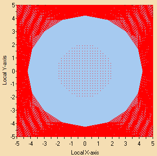
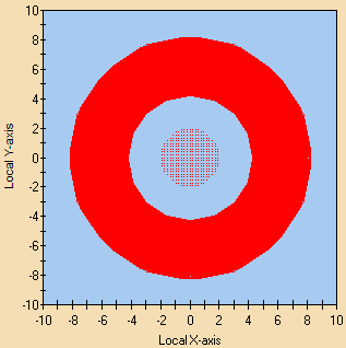
Let us now examine the individual beamlets at the same location using the Gaussian Ray Size Spot Diagram. This feature can be invoked directly after either of the two above approaches. Figure 2-13a shows the resulting Gaussian Ray Size Spot Diagram plot. Note that the beamlets overfill the Analysis Surface area. Open the Analysis Surface dialog box and reset the Scale factor to 5 and re-calculate. Now the area is large enough to encompass all of the beamlets as shown in Figure 2-13b. Note that editing the Analysis Surface does not require re-creating or re-tracing of the rays.
a) Figure 2-13. Gaussian Rays Size Spot Diagrams at Afocal entrance: a) Scale=2.5, b) Scale=5.
The thick red band surrounding the inner spot diagram results from drawing all the beamlets overlapping one another. An important point to note in Figure 2-13b is that the Gaussian beamlets extend beyond the 5 mm clear aperture of the first afocal lens. A rough guess of ~6mm for beamlet radius can be estimated from the graphic by measuring along the X-axis at Y=0 from the inner circumference of the red band on one side (-4) to the outer circumference on the opposite side (+8). This measurement would represent a beamlet on the right edge of the spot diagram.
Knowing that the beamlets extend beyond the lens clear aperture, it may seem reasonable to conclude that the secondary rays are clipped from the base ray. However, this is not the case. One of the fundamental rules of Complex Raytracing is: If the base ray intersects a surface then all of its secondary rays must intersect the same surface. FRED attempts to obey this rule by internally extending the surface based upon its mathematical definition. This presents no issue in a case such as this where the surface is spherical and is defined by the equation f(x,y,z)=x2+y2+z2+R2=0 where R is the surface radius of curvature.
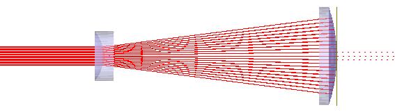
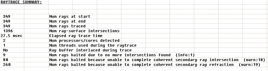
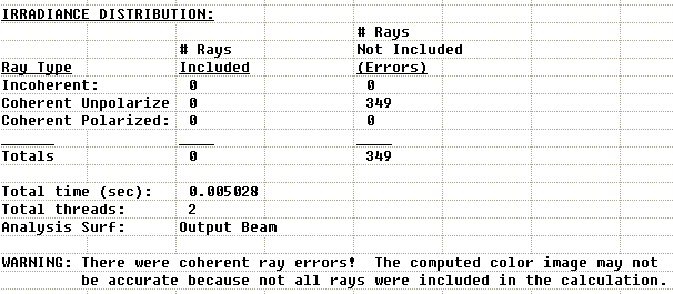
Having thoroughly examined the incident beam both at its creation plane and at the entrance of the afocal for the case where the beamwaist is located 5 meters away from the lenses, let us now return to the full raytrace as performed earlier and shown in Figure 2-7. A somewhat more revealing picture of the same trace is shown in Figure 2-14. This time, attention should be direct to the afocal exit aperture. The graphic seems to indicate that most of the rays stopped tracing once they intersected the second surface of the second lens leaving only a few to continue their journey beyond the lens. FRED offers information relevant to this situation in the Raytrace Summary printed in the Output Window as shown in Figure 2-15. The output indicates warnings for 340 of the 349 rays. The two distinct warnings indicate serious errors which cause these coherent rays to terminate propagation. As a result, an irradiance calculation at the afocal output is no longer valid. In fact, attempting an irradiance calculation using the Analysis Surface Output Beam produces a null result as shown in Figure 2-16. While a detailed explanation is beyond the scope of this tutorial, the Field Resampling feature is now presented as a method for circumventing such problems.
Figure 2-14. Raytrace through afocal showing ray failures.
Figure 2-15. Raytrace Summary in Output Window after trace
Figure 2-16. Output Window printout when irradiance calculation is attempted after raytrace.
Field Resampling
Let us summarize the situation as it currently stands. A Laser Beam (00 mode) type Source Primitive with 1/e2 half-width of 1 mm located at the entrance aperture of simple Galilean afocal telescope was traced through the system and the irradiance at the exit aperture was easily calculated. This source was then shifted 5 meters away from the telescope and re-traced. It was found that, in this case, we were unable to calculate the irradiance at the telescope output due to coherent ray errors. We noted as shown in Figure 2-13 that the individual Gaussian beamlets comprising the source had diverged significantly in traversing the 5 meters to the point where they were on the order of or larger than the lens aperture. While this may not be the deciding factor in the failure to calculate output irradiance, we may suspect that this is one of the contributing factors.
This section of the tutorial introduces FRED's Field Resampling feature. A more detailed description of this feature and its application to a more extreme case is provided as an example in the Help documentation. The Field Resampling feature computes the scalar field at the telescope entrance, deletes existing rays and creates a new set of rays which more accurately sample the optic aperture. Its application in this example is intended to eliminate generation of coherent ray errors and allow the irradiance at the telescope exit to be accurately calculated. With the Field Resamping feature, the sampling takes place in the plane of a selected Analysis Surface and creates a new coherent beamlet at the center of each of its pixels. The beamlet diameter is equal 1.5 times the pixel dimension (the factor of 1.5 is the overlap factor discussed in the Basic section). The amplitude and phase of each new ray is based upon the scalar field calculated in the corresponding pixel. The ray trajectories are adjusted to be normal to the wavefront.
Selection of pixel size is dictated by two competing constraints. At one extreme, the pixels should not be so small as to generate beamlets with large divergence angles. This is equivalent to Δx = (2/1.5)ω0 >>λ. At the other extreme, the pixels should not be so large as to have a pixel-to-pixel phase shift of greater than π. In all but the most extreme cases, this represents a rather large range of suitable pixel sizes. It is appropriate in this case to simply choose the pixel size so as to create new beamlets equal in size to those of the initial beamlets. With this objective in mind, open the Analysis Surface Irradiance at laser source dialog and disable Autoscale. Set the Analysis Surface dimensions equal to that of the lens aperture [XMin =-5, XMax =+5, Scale=1]. Since the initial source grid spacing was 21 rays across an aperture of +/- 2mm (see Figure 1-5), set the number of pixels in X & Y to 51. Recall that the origin of afocal coordinate system is at the vertex of the first lens. Therefore, it is necessary to shift the Analysis Surface just far enough to the left (Z=-2mm) so that it is clear of the lens. This must be done to ensure that all rays created in the Analysis Surface plane are immersed in the same material; in this case, Air. Figure 2-17 below shows the dialog for Irradiance at laser source properly configured.
Figure 2-17. Analysis Surface Irradiance at laser source dialog configured for Field Resampling.
The next step will be to trace the source rays to the entrance surface of the afocal using the Advanced Raytrace dialog configured as in Figure 2-12. After the trace, open the Field Resampling dialog from the Main Menu Raytrace>Spatially Resample Field. First, select the Analysis Surface Irradiance at laser source which was configured appropriately above. Select the Reference Wavefront option Parameters Determined by Fitting leaving the default values of 150 for the Number of Guesses. Under the Ray Generation options, set the Relative power cutoff to 1e-03 and check both the As calculated and With reference wavefront subtracted from phase boxes under Display Pre-resampled Field. The Field Resampling dialog with these settings is shown in Figure 2-18.
Figure 2-18. Field Resample dialog configured for ray creation at afocal entrance.
When the OK button is pressed, several things occur in series. FRED first calculates the scalar field in the plane of the designated Analysis Surface and will display the result in the Chart Viewer as directed by the Display Pre-resampled Field setting. Next, the existing rays are deleted and replaced by the new rays. The new rays have been created and are waiting to be traced. Figure 2-19 shows the Coherent Scalar Field Energy calculated from the initial rayset. Note that the Energy profile is of negligible amplitude outside of a circle of radius 2mm. It is recommended that the phase of this field be examined to ensure a smooth profile with no ambiguities or discontinuities. Right-click in the left portion of the Chart and select the option Show Field Phase. Figure 2-20 shows the corresponding Phase profile. Discontinuities are noted in the phase profile but these occur beyond the radius for which the energy drops to negligible values. A smooth phase profile is observed across the central portion of the beam.
Figure 2-19. Coherent Scalar Field Energy calculated by Field Resample feature.
Figure 2-20. Coherent Scalar Field Phase calculated by Field Resample feature.
At this point, the new rays have been created and are ready to be traced. Since these rays now exist, they must be traced as Existing rays by using one of the following methods:
1.From the Main Menu, Raytrace>Trace Existing and Render 2.Keystroke Ctrl+Shft+F11 3.Raytrace Toolbar button
Proceed by navigating back to the 3D View and trace the existing rays as indicated. This should produce the view shown below in Figure 2-21. Note that the rays overfill the second lens to a small extent.
Figure 2-21. Resampled rayset traced through the afocal.
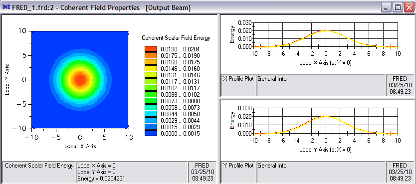
This leaves one final step; calculating the beam profile at the afocal output. Instead of using the Irradiance feature, try the Scalar Field feature with the Analysis Surface Output Beam. Recall that a Scalar Field calculation also provides access to a Wavefront profile by right-clicking in the Chart. Figures 2-22 and 2-23 show the Energy and Wavefront profile, respectively.
Figure 2-22. Scalar Field Energy at afocal output after Resampling.
Figure 2-23. Scalar Field Phase at afocal output after Resampling.
In the Advanced section of this Tutorial, the process of Resampling shown above will be implemented in FRED's scripting language.
[1] Arnaud, Jacques, “Representation of Gaussian Beams by Complex Rays”, Applied Optics, Vol. 24, No. 4, p. 538-543, Feb 1985
|
.png)
.png)
.png)
.png)
.png)
.png)