|
Specular directions at which the BSDF for the selected scatter model(s) will be plotted. Values may be entered using one of the four interpretations below and can include white-space and grouping characters (such as "()", "{}" and "[]"). Commas are interpreted as the separator between associated X,Y angle pairs but no whitespace is allowed before or after the comma. Values that are not separated by commas are considered to be a Y component with an implied X component of 0. Interpretation of the values entered is indicated by a two letter prefix in front of the values as indicated below.
Note: Specification of angle pairs is only useful when the scatter model(s) being plotted are anisotropic (i.e. the BSDF changes as the scattering surface is rotated about its surface normal). Only the Scripted and Extended Scripted scatter models have the capability of supporting anisotropy. Requesting angle pairs with isotropic scatter models will simply result in a rotation of the scatter function around the direction cosine circle without a change in the magnitude of the BSDF.
List of Y angles in degrees
Entering a list of single angles specifies the specular directions in degrees along the Y axis. This option is sufficient for displaying isotropic scatter models.
Usage examples:
Three specular angles along the Y axis:
0 30 75
In the additional conventions that follow below, the specular direction list can be supplied with single stand-alone values and/or value pairs. A single stand-alone value indicates the Y component of the specular direction with an X=0 component being implied. Value pairs are indicated using the format, "Y,X", where only a comma exists between the two values and are used to query the BSDF with specular directions off the Y-axis.
Direction sines
Indicated by the prefix, "ba" (for beta-alpha), this convention allows the user to specify the specular directions as direction sines. Single values indicate the Y direction sine and value pairs indicate the specular direction as ( sin(qy), sin(qx) ).
Usage examples:
Two specular directions along the Y-axis at 30 degrees and 60 degrees
ba 0.5 0.866
Three specular directions, one along the Y axis at 30 degrees, one along the X axis at 30 degrees and one in the XY plane at Y=45,X=45 degrees
ba 0.5 (0,0.5) (0.707,0.707)
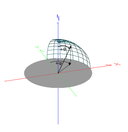
Spherical coordinates
Indicated by the prefix, "tp", this convention allows the user to specify the list of specular directions in a spherical coordinate system. Directions are specified as (q,f), where q is the polar angle (q=0 is aligned to the Z axis of the scatter model's local coordinate system) and f is the azimuthal angle (f=0 is aligned to the +Y axis). Positive azimuthal angles rotate clockwise from +Y to +X. A graphic of the coordinate system convention is shown below.
Usage examples:
Three specular directions along the Y axis at 20, 40 and 60 degrees
tp 20 40 60
Four specular directions, one along the Y-axis at 30 degrees, one along the X-axis at 30 degrees, one at (q,f) = (30,-30) and one at (q,f) = (30,60).
tp 30 (30,90) (30,-30) (30,60)
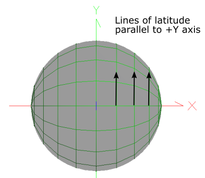
Theta-Theta Projection
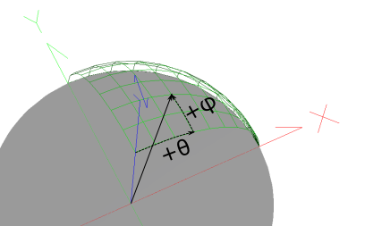
Indicated by the prefix, "tt", this convention uses a spherical coordinate system that is rotated so that the projected latitude lines of the spherical coordinate system are parallel to the +Y axis. This projected view is shown in the image below.
Directions are specified as (f,q) as shown in the image below. This convention allows the specular directions to be varied along the Y axis by holding q at a fixed value.
Usage examples:
Four specular directions, one along the X axis at 30 degrees, one along the -X axis at 30 degrees, one at (f,q) = (-10,30), and one at (f,q) = (20,30).
tt (0,30) (0,-30) (-10,30) (20,30)
Six specular directions with a fixed q = 10 degrees. Specular directions are moving along the Y axis with f=0, 15, 30, 45, 60, 75 and 89.5
tt (0,10) (15,10) (30,10) (45,10) (60,10) (75,10)
|