|
Description
The Digitization Tool (or Digitizer) allows the user to digitize data points from a graph, plot, lens drawing, etc. from an image file. The user can import an image file in a number of different image file formats including BMP (bitmap), PCX (PC Paintbrush), JPEG, PNG, GIF, TGA (Targa), or TIF. From the image file, the user will identify the graph origin, the X-axis scale, and the Y-axis scale and select data points for acquisition.
Depending on where the Digitization Tool was called from, the exported data will be formatted appropriately. The following data formats will be exported given the calling dialog:
Sampled Materials - refractive index vs. wavelength
Source Wavelength list - weight vs. wavelength
Detailed Source Directional Power Apodization - directional apodization (Sampled as a function of spherical angles) in terms of weight vs. polar angle
Detailed Source Ray Direction - "Randomly according to intensity distribution" generates ray directions according to weighting values in spherical coordinates
Segmented Curve - XY, YZ or XZ coordinate pairs
Sampled Coating - transmission/reflection vs. wavelength
Spectra - sampled wavelength vs. value
Navigation
The Digitizer can be accessed in the following ways:
Sampled Coating - Right mouse click in the spreadsheet area of the Sampled Coating specification and select "Digitize Reflection Curve" or "Digitize Transmission Curve" from the list menu.
Sampled Material - Right mouse click in the spreadsheet area of the the Sampled Material specification and select "Digitize Material Index" from the list menu.
Segmented Curve - Right mouse click in the spreadsheet area of the Segmented curve points specification and select "Digitize X-Y Data (X horizontal, Y vertical) From Image", "Digitize Y-Z Data (Y vertical, Z horizontal) From Image", or "Digitize X-Z Data (X vertical, Z horizontal) From Image" from the list menu.
Source Wavelength list - Right mouse click in the source wavelength list and select "Digitize From Image" from the list menu.
Detailed Source Directional Power Apodization - With type "Sampled as a function of spherical angles", right mouse click in the spherical angle apodization spreadsheet area and select "Digitize Curve" from the list menu.
Detailed Source Ray Direction - With the type "Randomly according to intensity distribution", right mouse click in the spreadsheet area and select "Digitize Curve" from the list menu.
Spectra - Right mouse click in the spreadsheet area of a sampled spectrum and select "Digitize Curve" from the list menu.
Controls
|
Control
|
Inputs / Description
|
Defaults
|
|
Select Image
|
Allows selection of an image file from disk.
|
|
|
Select X, Y Min Point
|
Sets the origin of the X- and Y-axes on the image.
|
|
|
Select X Max Point
|
Sets the maximum point on the X scale.
|
|
|
Select Y Max Point
|
Sets the maximum point on the Y scale.
|
|
|
X Origin
|
Sets the value of the origin point on the X scale.
|
0
|
|
Y Origin
|
Sets the value of the origin point on the Y scale.
|
0
|
|
X Max
|
Sets the value of the max point on the X scale.
|
0
|
|
Y Max
|
Sets the value of the max point on the Y scale.
|
0
|
|
Log X Axis
|
Defines the X-axis as a logarithmic axis. Values for the X Origin and X Max are limited to positive, nonzero values.
|
Unchecked
|
|
Log Y Axis
|
Defines the Y-axis as a logarithmic axis. Values for the Y Origin and Y Max are limited to positive, nonzero values.
|
Unchecked
|
|
Image Coordinates
|
Specifies the location of the cursor in bitmap coordinates, relative to the point X=0, Y=0 at the upper left corner of the image.
|
(0, 0) is at the upper left corner
|
|
User Coordinates
|
Specifies the location of the cursor in the coordinate system you define. Shown as undefined until Data Selection Mode chosen.
|
Undefined
|
|
Image
|
Displays the image selected for Digitization.
|
|
|
|
|
Select Data
|
Toggles Data Selection Mode if all requisite parameters have been specified correctly.
|
|
|
Export Data
|
Exports data selected to the dialog that brought up the Digitization Tool (for example, the sampled materials edit dialog).
|
|
|
Save to File
|
Saves selected data in a text file in x, y format, one point per line.
|
|
|
Help
|
Brings up this help article.
|
|
|
Cancel
|
Dismisses the dialog without exporting any data to the coating or material.
|
|
Application Notes
Step by step guide to using the digitization tool
The following example uses the reflectivity plot for an AR coating to digitize the reflectivity vs. wavelength. These steps should be followed in order to digitize the data properly.
|
1.
|
|
Select the image to be digitized by clicking the "Select Image" button in the Digitizer dialog box.
.bmp)
|
|
2.
|
|
Click the "Select X, Y Min Point" button and then left mouse click on the graph at the point where the X and Y axes cross. A symbol will mark the selected location. NOTE: As long as the "Select Data" button has not been selected, the X, Y minimum point can be changed. Otherwise, the dialog will have to be closed and the process started over in order to acquire a new X, Y Min Point.
|
|
3.
|
|
Enter the graph or plot coordinates of the X, Y Min Point in the boxes labeled "X Origin" and "Y Origin". In this example the axes cross at X = 400 nm and Y = 0, so the X Origin value should be entered as 0.4 and the Y Origin value should be entered as 0.
|
|
4.
|
|
Click the "Select X Max Point" button and then left mouse click on the maximum X axis coordinate. NOTE: The point does not have to be the max value on the X axis, it just needs to be a point that can be numerically identified on the graph. The X maximum point selection can be changed as long as the "Select Data" button has not been clicked. Once the "Select Data" button has been pushed, the X Max Point can no longer be changed.
|
|
5.
|
|
Enter the graph coordinate for the point selected on the X axis in the box labeled "X Max". In this example, the selected X Max Point is 700 nm, so the X Max value should be entered as 0.7.
|
|
6.
|
|
Click the "Select Y Max Point" button and then left mouse click on the maximum Y axis coordinate. NOTE: The point does not have to be the max value on the Y axis, it just needs to be a point that can be numerically identified on the graph and perpendicular to the line connecting X, Y Min and X Max. Failure to choose the Y-axis perpendicular to the X-axis will result in improper digitization of data values.
|
|
7.
|
|
Enter the graph coordinate for the point selected on the Y-axis in the box labeled "Y Max". In this example, the selected Y Max Point is 2.5.
|
|
8.
|
|
Click the "Select Data" button and start acquiring data by left mouse clicking on the appropriate data points in the graph. Each selected data point will be marked with a symbol. The data points are not sorted before being loaded back into FRED, so they should be selected in a reasonable order. In this example the data points are selected in order of increasing wavelength.
|
|
9.
|
|
Either save the data to a text file by clicking the "Save to file" button or export the data directly into the FRED dialog that called the digitizer by clicking the "Export Data" button.
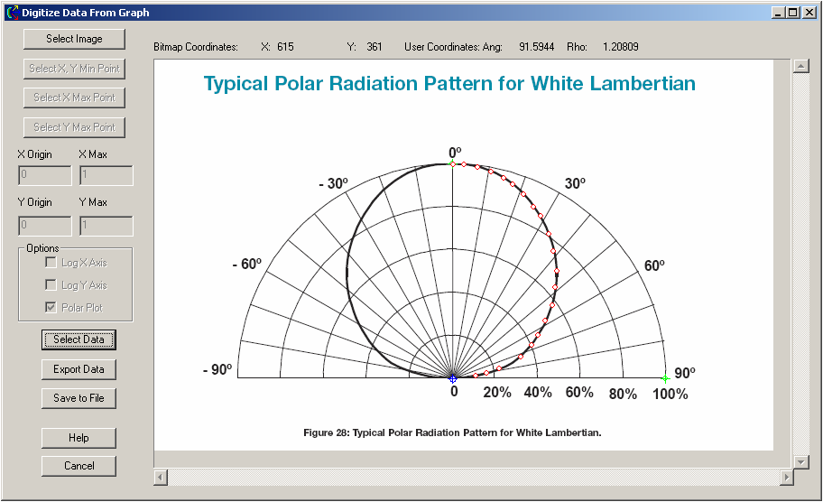
In the following image, the X, Y Min Point is marked by a blue icon, the X Max Point and Y Max Points are marked by green icons and the sampled data points are marked by red circles.
.bmp)
|
Deleting data points
A right mouse click deletes previously selected data points from the digitizer.
Bitmap and user coordinates
Current bitmap pixel coordinates and interpreted "user" coordinates based on the X,Y Origin and Min/Max points are displayed at the top of the digitizer window. It is a good idea to check the "user" coordinates during data acquisition to make sure that the specified values make sense.
Exporting digitized data
If you would like to save the acquired data to a ASCII text file press the "Save To File" button. This can be useful when the data is to be used in multiple models or to save the data for re-use at a later time.
Acquired data can be exported directly to the FRED dialog which called the digitization tool by clicking the "Export Data" button.
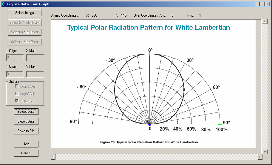
Polar plots
Digitization of data from polar plots requires proper marking and scaling of the fiducial points. In polar coordinates the following transformation is used:
x = r sin(j) y = r cos(j)
In the image below, r has values from 0 to 1 and j has values from 0 to 90 degrees. Therefore, y has values from 0 to 1 and x has values from 0 to 1.
|
Copyright © Photon Engineering, LLC
|
|