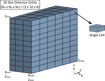
The 3D Box is a specialized type of detector entity which records the flow of power as it propagates through box's volume. The volume is composed of a number of 3D cells which allow the spatial distribution of power transfer between adjacent cells to be captured during the raytrace. In the diagram below, a 3D Box has been defined with 3 cells in X, 10 cells in Y and 6 cells in Z.
Individual surfaces of the detector entity have the ability to intersect rays during the raytrace, though they are optically non-interacting (i.e. they have no optical effect on the rays). This means that walls of the 3D box can be arbitrarily sized to enclose (partially or completely) other surface geometries in the system.
There are three quantities calculated per cell by the 3D Box detector entity: •InFlux - Total power entering the cell •OutFlux - Total power leaving the cell •AbsorbedFlux - Difference between InFlux and OutFlux and including pre/post trace offsets (see below)
For simplicity we clarify the meaning and method of these quantities below using a two dimensional cell model, though the same procedure applies when the cell is extended into three dimensions. In the image below we show two cases of ray intersections with a single cell in the 3D box detector entity; on the left the case for a single ray and on the right the case for multiple rays.
Per cell, the power absorbed is simply the power input into the cell less the power leaving the cell. Similarly, the flux into the cell (InFlux) is the summation of the power on all surfaces coming into the cell and the flux out of the cell (OutFlux) is the summation of the power on all surfaces leaving the cell. For the simple case shown above of a single ray passing through a single cell of the 3D box, there is total input flux of fin, total output flux of fout and the difference between the two results in the absorbed flux. As shown on the right in the image above, the calculation proceeds the same for the case where multiple rays are passing through a cell in the 3D box. In this case, we simply sum over all rays incident on the cell surfaces to get the InFlux value, sum over all rays leaving the cell surfaces to get the OutFlux value and the difference between the two is the AbsorbedFlux value.
To clarify further, we describe the scenario where a cell in the 3D Box partially encloses an optical surface. In this case we explicitly label the individual surfaces of the cell as A, B, C and D, though the individual cell surface calculations are transparent to the user when using this feature in FRED. The optical surface has a coating applied which is 95% transmitting and 3% reflecting.
For the two input rays shown, only cell surfaces A and D have input flux and the resulting cell InFlux is therefore the summation of the input flux from these two surfaces. Only cell surfaces B and C have output flux and the resulting cell OutFlux is therefore the summation of the output flux from these two surfaces. The cell's absorbed flux is the difference between the InFlux and the OutFlux, which in this case leaves 2% of the power from ray #1 within the cell (ray #2 undergoes total internal reflection at the interface).
Embedded Sources and Halted Rays In the description above regarding the calculation of AbsorbedFlux from the InFlux and OutFlux cell quantities we have used the case where the sources are created outside of the 3D Box volume and all rays are exiting the volume by the end of the raytrace. Controls are provided on the 3D Box detector entity to allow the user to address the cases where a source is created within the 3D Box or when rays are halted inside of the 3D Box at the end of the raytrace (or a combination of both scenarios).
Embedded Sources How does having a source starting inside of a cell of the 3D Box affect the resulting calculation of AbsorbedFlux? If the source starts within a cell of the 3D Box, then its flux is not counted in the InFlux calculation (the rays never crossed the cell walls coming into the cell) but its flux is counted as the rays leave the cell. The net result is that the AbsorbedFlux value in the source's starting cell is negatively biased by the amount of the source's flux. If the user wants to remove the negative bias due to the source's starting flux, the InclPreTrace boolean can be set True. This has the effect of adding the source's flux as a positive offset in the AbsorbedFlux calculation.
Halted Rays During a raytrace, a given ray may be stopped on a surface for a variety of reasons (ex. due to raytrace control settings). Similar to the case where you have an embedded source, these halted rays are counted on the InFlux value but not on the OutFlux value. The result of these rays halting within a cell is that the cell's AbsorbedFlux value is positively biased by the ray's flux. If the user wants to remove the positive bias due to the halted ray's flux, the InclPostTrace boolean can be set True. The halted ray's flux is then added as a negative offset in the cell's AbsorbedFlux calculation.
To illustrate these controls, consider an extension of the previous example where we have a source embedded within a single cell that also contains a coated surface interface. The coating property on the surface is defined such that R+T<1 and the raytrace property on the surface will leave behind an Absorbed Ray having flux 1-(R+T) upon interaction. The resulting AbsorbedFlux calculation for the four combinations of the InclPreTrace and InclPostTrace flags are provided below as a numerical example to help clarify their application.
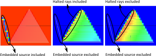
As a final example illustrating the concept and impact of applying offsets to the 3D Box calculation, we consider a 60 degree prism made out of a material having bulk absorption properties. The goal of the simulation is to display the AbsorbedFlux which is attributable to the material absorption of the prism. In the results below, we show the AbsorbedFlux values in the case with no offsets, pre-trace offsets (embedded source removed), and pre-trace and post-trace offsets (embedded source AND halted rays removed). When we choose not to apply offsets, we see that the source contribution uses most of the plot's dynamic range and obscures the absorption due to the prism material. When we apply only the pre-trace offsets, we see that rays halted on the entrance face of the prism are still accounted for and also use up the plot's dynamic range. Lastly, we apply both pre and post-trace offsets to remove the source and halted ray contributions and see that the AbsorbedFlux plot now displays the flux absorption due to the material loss.
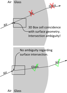
The individual cell walls of a 3D Box detector entity do intersect rays during the raytrace but have no optical properties (materials, coatings, scatter, etc.). This means that a 3D Box detector entity can be oriented and positioned within the model to enclose (partially or completely) other geometries in the system. However, surface coincidence must be considered when positioning the 3D Box within the model. Consider the two cases shown below:
If the 3D box has been positioned such that any surfaces of its cells are coincident with the geometry, the potential exists for the 3D box to induce incorrect results in the raytrace. This situation will typically be observed as material error warnings in the output window after the raytrace has completed.
The Identify Coincident Surfaces tool can be used to help identify whether any cell walls of a 3D Box detector entity may be coincident with other geometry in the system.
The 3D Box detector entity type is unique in how it handles coherent rays. Unlike the other detector entities, the 3D box ignores the coherent characteristics of the rays and bins them using the ray's incoherent data. Polarization properties are also ignored in the binning.
The flux values are recorded during the raytrace, so the power units in the cell data is always radiometric (either known or arbitrary). If a source has been defined in photometric units, the power in the cell data reflects the source power after converting from photometric to radiometric units.
The results of a 3D Box detector entity are automatically created and stored in an Analysis Results Node (ARN) on the object tree at the end of the raytrace. Cell data stored in the ARN can be visualized directly in FRED's 3D view by taking the following action: •Right mouse click on the ARN corresponding to the 3D Box detector entity and select "Display in Visualization View" from the context menu.
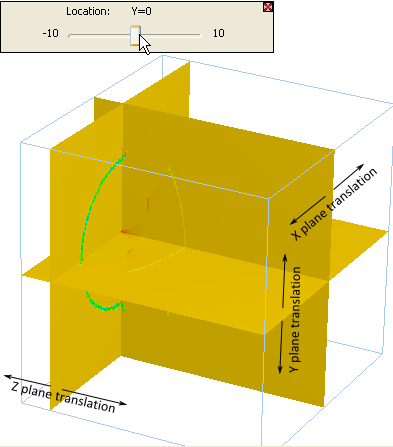
Visualization of the analysis results in the 3D view uses cutting planes which can be dynamically translated along their plane normals, allowing the quantity of interest to be displayed on the cutting planes anywhere within the volume. Once the analysis result has been displayed, any of the cutting planes can be activated for translation by double mouse clicking on the cutting plane of interest directly in the 3D viewer. This action puts the 3D viewer into a state which allows translation of the selected cutting plane and opens a slider bar dialog in the upper left corner of the visualization window. The cutting plane which was selected can be translated through the volume in the following ways: •Mouse wheel up/down •Keyboard up/down arrow •Keyboard page up/page down (steps 1/10 of volume width in the selected direction) •Explicit location set from the visualization view dialog (see below)
Until the slider bar dialog is dismissed using the red X in the top right corner of the dialog, FRED will not respond to any other mouse controls. An example analysis result displayed in the 3D view with the Y cutting plane activated for translation is shown below. Each plane has been annotated indicating is direction of translation.
The slicing planes are always displayed at the cell centers. If the location of the slicing plane has been explicitly set using the visualization dialog, then the location displayed in the 3D view will be the cell center nearest to the requested value.
When selected for display in the visualization view, the user is able to select the following visualization options for the 3D Box results:
The Analysis Results Node (ARN) created by a 3D Box detector entity can be exported from FRED into the following file formats: Lightweight Voxel (LMA) Absorption cell values are given in units of power*(1e-6)/mm3 InFlux and OutFlux cell values are given in raw power units Brick of Values (BOV) Absorption, InfFlux and OutFlux cell values are given in raw power units The BOV format will actually produce a set of 3 *.bov files and a set of 3 *.dat files, one each for the Absorbed, InFlux and OutFlux quantities. The *.bov file defines the construction parameters of the "brick" and the *.dat file contains the actual data for each cell. Visualization Toolkit (VTK) Absorption, InfFlux and OutFlux cell values are given in raw power units
Export of the ARN can be executed by right mouse clicking on the ARN corresponding to the 3D Box detector entity, then selecting "Export Data" from the context menu, and then choosing the desired file format.
A variety of data visualization packages exist which can read and display these file formats for data exploration and analysis. Some of these packages include: ParaView (Kitware) VisIt (U.S. Department of Energy, Advanced Simulation and Computing Initiative)
|
||||||||||||||||||||||||||||||||||||||||||||||||||||||||||||||||||||||||||||||||||||||||||||||||||||||