Directional synthesis is necessary for cases in which the paraxial limit imposed on individual beamlets would be violated if the gaussian beamlets were laid out on a rectilinear grid. For example, consider visible light incident upon a circular pinhole of diameter 10 mm in an opaque mask. An accurate spatial representation of the aperture would require a sampling frequency > 1 / l, in violation of the paraxial approximation (/o << 0.1). In the case of a directional synthesis, the field is synthesized from a collection of same-size beamlets originating from common points but with different directions, amplitudes and phases. The size of these beamlets is determined only by the Analysis Surface dimensions and wavelength, while the directional increment is determined by individual pixel size and the number of samples across the Analysis Surface; Dq = (Dx · N)-1 .
The accompanying FRED file, exampleSpatialFilter.frd, can be found in the <install dir>\Resources\Samples\Tutorials & Examples\ directory.
As a practical example, consider a spatial filter configuration in which a collimated flat-top beam is focused by a lens, passes through a pinhole and is re-collimated by a second lens. This layout is shown in the image below.
Note that the pinhole itself is not included in the geometry. A spot diagram at focus would reveal a ray grouping whose maximum extent is ±2 mm, so having an aperture greater that 4 mm diameter at focus would not block any of the base rays of the gaussian beamlets. It is important to note that regardless of the size of an aperture, if the base ray of a beamlet passes through the aperture all of its associated secondary rays also pass through the aperture. The converse is also true; if the base ray is blocked, so are all of its associated secondary rays. Since the rays being traced actually represent coherent gaussian beamlets, it should come as no surprise that the coherent summation of these rays at the pinhole plane has a greater spatial extent than the spot diagram. As expected, this lens produces an Airy disk at focus whose first dark ring has a radius of ~6.5 mm and thus, the pinhole must clip the field and not the rays.
To facilitate clipping by an aperture at focus, it is necessary to calculate the complex field in that plane. For this, a dummy surface must be placed at the pinhole position with an attached Analysis Surface. The choice of the Analysis Surface dimensions and number of divisions is key because for precise clipping it will be necessary to choose the Analysis Surface X and Y dimensions such that a pixel center falls at the desired radius. In addition, the Coherent Field Synthesis feature requires that the number of Analysis Surface divisions be 2n + 1 (65, 129, 257,... etc).
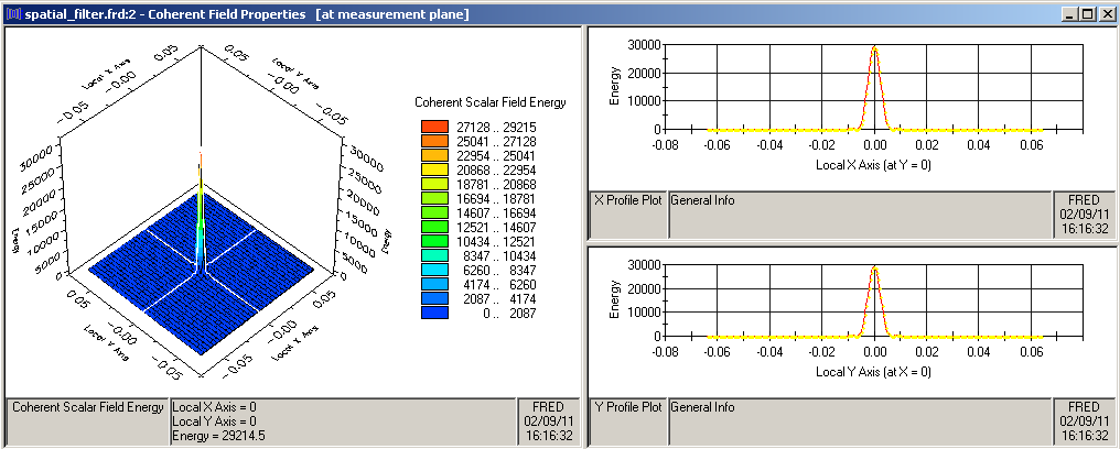
For this example, the pinhole radius will be equal to the radius of the first dark ring of the Airy pattern. To determine that precisely, we trace to the dummy plane and calculate the complex field (see images below). An estimate of the required window dimensions can be made using the formula, r = 1.22 l f/#, where r is the first dark ring radius, l is the wavelength and f/# is the f-number. For this configuration, l = 0.6328 mm and f/# = 8.6, giving r = 6.5e-3 mm. The profile of the focused beam is shown here for verification.
In order to effect the clipping due to the pinhole, a circular curve is first added to the Custom Element containing the pinhole plane. The radius of this circular curve is then 0.0065mm.
A second curve of type "Aperture Curve Collection" is also added to the pinhole Custom Element in order to facilitate application of the circular curve as a trimming entity. The circular curve must then be added to the Aperture Curve Collection and its Usage set to "Clear Aperture" so that the curve will trim away all portions of the field outside the limits of the circle.
The criteria for choosing the Analysis Surface dimensions and number of divisions will be to create a rayset that fills the aperture of the second lens when traced from the pinhole position, while at the same time providing a reasonable angular sampling of the subtended solid angle. The angle subtended by the lens is given by aTan(7.5 / 52) = 8.2°, so a reasonable Dq might be 0.25° to provide ~32 samples from center to edge and a gaussian beamlet radius L of approximately 145 mm. Given that the pinhole radius is to be 6.5 mm, the Dx increment should yield some integer number of pixels at that position. For instance, a pixel increment 0.5 mm over a distance of 145 mm yields 290 pixels. Since the number of pixels must be 2n + 1, a choice of 257 best matches. As a result, the beamlet radii L changes to 128 mm and the angular sampling increment adjusts to 0.28°, only about a 10% reduction in sampling. With the Analysis Surface settings adjusted appropriately, the resulting complex scalar field is shown below.
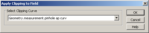
Trimming of the field with the pinhole curve is now accomplished directly from the Chart. Right-click in the Chart and select the option Coherent Field Operations>Apply Clipping to Field. This action will pop a dialog as shown below containing a dropdown list of allowed clipping curves. Select the Aperture Curve Collection created previously from this list and hit OK. FRED will apply the clipping aperture to the field and display the result in the Chart.
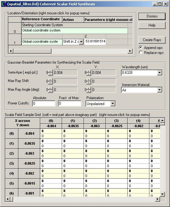
We can now proceed to the Coherent Field Synthesis dialog. Right-click in the Chart and select the option Coherent Field Operations>Synthesize Field. This action will open the Coherent Field Synthesis dialog as shown here and load the clipped field data into its sample grid area.
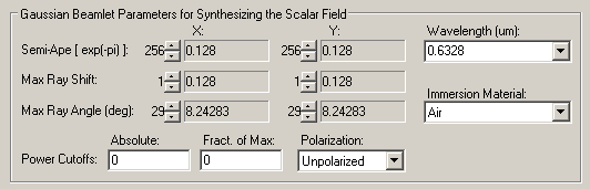
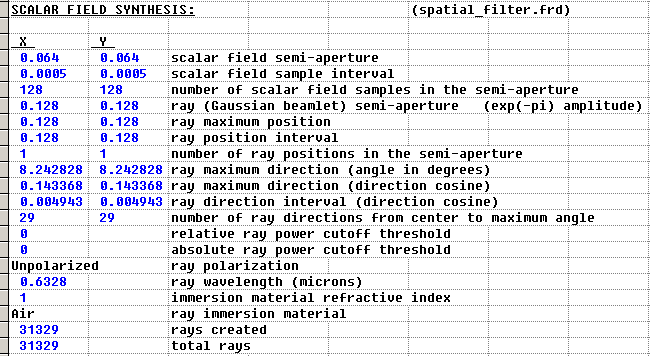
For a purely directional synthesis, we recommend that the beamlet semi-ape be set to its maximum value, which, in this case, is 256 samples (corresponding to L = 0.128 um). The Max Ray Shift should be set to 1 for both X & Y. This setting insures overlap of the individual beamlets as they propagate.
The maximum ray angle within the solid angle subtended by the lens uses 29 samples with an angle increment of 0.283°.
FRED can now be instructed to replace the rays used in the field calculation with the new synthesized rayset by selecting the "Replace Rays" option then clicking the Create Rays button at the top right of the Coherent Field Synthesis dialog box. Information concerning the rayset creation is printed to the Output Window. In this case, FRED created 3481 rays.
With the rays created, the Trace Existing or Trace Existing and Render button must be used. After tracing these rays an irradiance distribution is calculated on the plane to the left of the collimating lens. The resulting calculation is shown here contrasted with the unfiltered beam after collimation.
The accompanying script can be found in the Embedded scripts folder of the file exampleScriptingSpatialFiltering.frd located in the <install dir>\Resources\Samples\Tutorials & Examples\ directory.
Commands now exist for carrying out this task using the scripting language. The process is equivalent to the above steps and require the same calculations of proper Analysis Surface dimensions and pixel count as explained above.
The first step requires dimensioning six structures; T_RAY, T_ADVANCEDRAYTRACE, T_SYNTH_RAYS_FROM_FIELD , T_ENTITY, T_CIRCULARARC and T_APERTURECURVEOP. These structures are required for altering ray draw color, forcing a partial trace, synthesizing rays from the computed field and applying the aperture representing the pinhole, respectively. A number of other variables are also dimensions for use during the task. We recommend dimensioning ALL variables used in your script to avoid any possibility of improper initialization. These global variables define the pinhole radius and maximum ray angles for synthesis and are assigned values in the Edit/View Global Script Variables dialog found on the Tools menu for easy access from the FRED document without the need to edit this script.
Dim ray As T_RAY Dim tr As T_ADVANCEDRAYTRACE Dim sf As T_SYNTH_RAYS_FROM_FIELD Dim ent As T_ENTITY, crv As T_CIRCULARARC Dim ap(0) As T_APERTURECURVEOP Dim xmin As Double, xmax As Double, ymin As Double, ymax As Double Dim wav As Double, R As Integer, G As Integer, B As Integer
Sub Main
pi#=Acos(-1) deg#=pi/180
InitAdvancedRaytrace tr tr.suppressSummary=True
idm&=FindFullName("Geometry.pinhole.plane") ids&=FindName("Source 1") ida1&=FindName("at pinhole plane") ida2&=FindName("exit plane") idth&=FindFullName("Geometry.final.viewing plane") idcrv&=FindFullName("Geometry.pinhole.circle") idapcrv&=FindFullName("Geometry.pinhole.circleApCrv")
Next, we ensure that the input source is traceable before beginning the raytrace and pick up its wavelength. This is followed by lines that set the pinhole size g_pholerad (variable defined in the Global Script Variables dialog) and ensure that the curve is part of the Aperture Curve Collection. Note: An Update is required after any change to the model geometry or source settings.
SetTraceable ids,True wav#=GetSourceIthWavelength(ids,0)
GetCircularArc idcrv,ent,crv crv.startX=g_pholerad : crv.startY=0 : crv.endX=g_pholerad : crv.endY=0 SetCircularArc idcrv,ent,crv GetApertureCurve idapcrv,ent,ap ap(0).curv=idcrv : ap(0).action="ClearAperture" SetApertureCurve idapcrv,ent,ap Update Rays are now trace to the pinhole plane using an Advanced Raytrace.
tr.stopSurfID=idm cnt&=AdvancedRaytrace(tr)
The Scalar Field is now computed then stored in a file for the purpose of clipping and stored in an ARN for the purposes of determining the data dimensions and resolution. Once info has been read from the ARN, it is immediately deleted.
fname1$=GetDocDir() & "\unaperturedfield.fgd" cnt=ScalarFieldToFileAS(ida1,fname1) idarn&=ARNCreateFromFile(fname1,"unaperturedfield") xnum&=ARNGetAAxisDim(idarn) ynum&=ARNGetAAxisDim(idarn) ARNGetAAxisRange idarn,xmin,xmax ARNGetAAxisRange idarn,ymin,ymax ARNDelete idarn The pinhole aperture is applied to zero the field outside the pinhole radius using the ClipFieldInFile command:
fname2$=GetDocDir() & "\clippedfield.fgd" ClipFieldInFile idapcrv,fname1,fname2 Rays from the original source are no longer need and MUST be deleted. It is also of vital importance to turn off the original source. Once again, an Update is required.
DeleteRays 'delete original source rays SetTraceable ids,False 'turn off existing source Update
The synthesis structure T_SYNTH_RAYS_FROM_FIELD must now be setup to produce the desired rayset. The user must also set up the maximum angle for which rays will be created. In most cases, this should be set to correspond to the angle subtended by the next optic as measured from the source location. In this example, the maximum angles are set in the Edit/View Global Script Variables dialog. The only other information required are the spatial frequency deltas determined by Analysis Surface pixel count and size.
omegax#=1/(xmax-xmin) omegay#=1/(ymax-ymin)
The values for members XSemiAp and YSemiApe are set based upon the values given from g_thetax and g_thetay, variables defined in the Global Script Variables dialog. Note that the wavelength is given in microns while the spatial frequency is in inverse mm; thus the factor of 1e-3 in the definitions of XMaxRayAngle and YMaxRayAngle members. The subroutine setsynth is included below.
sf.XMaxRayAngle=Int(Sin(g_thetax*deg)/(wav*1e-3*omegax)) sf.YMaxRayAngle=Int(Sin(g_thetay*deg)/(wav*1e-3*omegay)) sf.XSemiAp=xnum-1 : sf.YSemiAp=ynum-1 Print "Adjusted max XY ray angle " & Asin(sf.XMaxRayAngle*wav*1e-3*omegax)/deg setsynth
With the T_SYNTH_RAYS_FROM_FIELD set and the Scalar Field file available, rays can now be synthesized for the field apertured by the pinhole with the CreateRaysFromScalarFieldFile command. These rays are located in the coordinate of the pinhole plane. Note that these rays are now "Existing" rays
cnt=CreateRaysFromScalarFieldFile(fname2,sf,0) These new rays will have a white draw color. Therefore, a loop is included to set the ray draw colors from their wavelength. 'set ray color from wavelength WavelengthToRGB wav,R,G,B success=GetFirstRay(cnt,ray) While success ray.colorR=R : ray.colorG=G : ray.colorB=B SetRay cnt,ray success=GetNextRay(cnt,ray) Wend
The newly synthesized rays is now traced through the remainder of the optics, namely the second lens. The member stopSurfID is now set to "Don't Care" (-1) and the traceActiveSources flag is set to False since the rays to be trace already exist.
tr.stopSurfID=-1 tr.traceActiveSources=False cnt=AdvancedRaytrace(tr) Finally, the Irradiance is calculated on the observation plane and displayed in the Chart Viewer.
End Sub
Subroutine setsynth set the remaining members of T_SYNTH_RAYS_FROM_FIELD.
Sub setsynth sf.OverlapFactor=1 sf.PowCutoffAbs=0 sf.PowCutoffFract=0 sf.XMaxRayShift=1 sf.YMaxRayShift=1 sf.material=0 sf.ReverseDir=False End Sub
|
.png)
.png)
.png)
.png)
.png)

.png)
.png)
.png)