Once variables and merit function aberrations have been defined, the optimization process can proceed by one of several methods. The goal of the optimization algorithm is to explore the variable space within the user specified limits and modify the variable values iteratively in order to drive the merit function value towards a minimum. Specifying how the optimization routine explores the variable space is done using the Method portion of the optimization's Define/Edit dialog. In general, there are two methods for exploring the variable space; globally or locally. In a global type optimization, the broader variable space is explored and merit function minimization proceeds using one or more variable configurations from that search. In a local type optimization, the variable space in the region of the starting configuration is explored and merit function minimization proceeds from that starting configuration. The implicit assumption of local optimization is that the starting configuration lies near to the optimal configuration in the merit function space. A listing of the available local and global optimization methods is provided below:
This feature can be accessed by selecting Optimization > Define/Edit: Method from the menu.
The Simplex method of optimization1,2,3,4,5,6 is a geometric approach to optimization and is akin to a ball rolling down a hill, where the hill is analogous to the merit function and the ball indicates points that are sampling the variable space. The number of points in the simplex is the number of dimensions plus one, where the simplex undergoes reflection, expansion, and two forms of contraction to search the variable space. The simplex method is very robust, meaning that there is confidence in convergence even in systems with stochastic (i.e., random) noise. However, noise is always present in ray tracing of non-sequential optical systems due to limitations in discrete ray sampling. Additionally, the simplex method does not employ derivatives, which are typically unavailable in non-sequential analysis. Because of the lack of derivative information, the simplex method will proceed in a slower manner than other algorithms which take advantage of derivative information to guide the variable search.
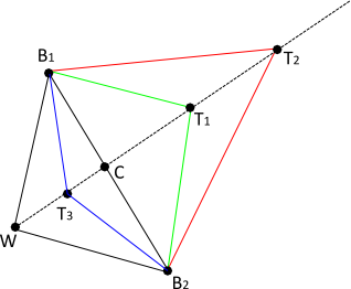
Although the simplex can represent an arbitrary n-dimensional function, the 2-D case serves a useful illustration of the simplex method. Consider a 2-D function which has been sampled at three locations within the variable space to form a triangle, which is the simplex (shown below). These points can be evaluated as best (B1), second best (B2) and worst (W). In order to improve the simplex, we wish to move the worst point to a new position and improve the merit function evaluation. Three operations are potentially performed on the simplex to move point W, reflection about B1B2, an expansion and a contraction. The following steps would be taken:
[1] W. H. Press, B. P. Flannery, S. A. Teukolsky, and W. T. Vetterling, Numerical Recipes in C (Cambridge U. Press, Cambridge, England, 1992), pp.395-455. [2] Nelder J.A., Mead R., 1965, Computer Journal, 7, 308 [3] R. J. Koshel, "Simplex optimization method for illumination design," Opt.Lett. 30, 649-651 (2005) http://www.opticsinfobase.org/abstract.cfm?URI=ol-30-6-649 [4] R. J. Koshel, Proc. SPIE 4832, 270 (2002). [5] http://en.wikipedia.org/wiki/Simplex_algorithm [6] http://en.wikipedia.org/wiki/Nelder-Mead_method
Simulated Annealing is a pseudo-global optimization algorithm which has its foundations in thermodynamics. Consider a high temperature liquid metal whose molecules are able to freely move about. In thermal equilibrium, the energy of the system at temperature T has energy which is distributed probabilistically among all different energy states E according to the Boltzmann probability distribution: Probability(E) ~ e(-E/kT) If the molten metal is cooled slowly, the constituent molecules lose mobility. If the cooling is slow enough (annealing), the metal forms a crystalline structure having the minimum energy configuration. Unlike the standard Simplex, this method allows for the probability of a step upward in energy for any given iteration. Accepting only downward steps in energy is equivalent to quenching the metal into a polycrystalline configuration, which is the approach that the standard Simplex method takes. In this manner, the Simplex method is a local optimization strategy since there is no probability of taking an upward step to escape from a local minimum energy configuration.
In its relation to optimizing the FRED system model, the temperature T is representative of the merit function value at a given energy level. At any given temperature, the simplex undergoes random thermal tumbling as it searches the current energy level. When it has finished its search, the temperature is reduced and another search at the next energy level proceeds. Because the simplex undergoes random perturbations during the search, it has the opportunity to explore many local minimum during any given iteration. As the temperature is reduced, the number of local minimum being explored decreases and the algorithm (ideally) settles into the global minimum.
True to its name, the success of the Simulated Annealing optimization method depends heavily on annealing schedule. That is, the starting temperature, temperature reductions and the number of iterations at each energy level determine whether or not an optimal configuration is found. Determining the proper annealing schedule for a given optimization problem will require some trial and error on the part of the user. However, some suggestions for starting temperature and annealing schedule have been built into the dialog as default parameters. For example, the Auto option for choosing the starting temperature will compute the merit function value for a number of starting configurations and set the starting temperature such that the optimization has an 80% chance of stepping over the largest merit function value found. Additionally, the temperature reduction factor is set at 0.9 in accordance with [1]. Regarding the convergence criteria, each option applies to a single temperature in the annealing schedule. For example, a given temperature may undergo N iterations according to the "After iterations" convergence criteria. After the iterations have completed, the temperature is reduced and another N iterations of the simplex are performed. Once the minimum temperature of the annealing schedule has been reached, the optimization undergoes one final local standard Simplex optimization. The user may start with 10-100 iterations specified in the "After iterations" setting when Simulated Annealing is used. Keep in mind that the algorithm has its best chance for success when the temperature is cooled slowly, but you also need to get a result in a finite amount of time!
[1] B. Flannery, W. Vetterling, S. Teukolsky, W. Press. Numerical Recipes: The Art of Scientific Computing (3rd Edition). New York: Cambridge University Press, 2007.
Optimize - Merit Function Aberrations Optimize - Sensitivity Analysis
|
|||||||||||||||||||||||||||||||||||||||||||||||||||||||||||||||||||||||||||||||||||||||||