This Advanced section will draw upon material introduced in the Intermediate section to 1) demonstrate implementation of the Field Resampling technique in FRED's scripting language, and 2) optimize the afocal lens performance for different locations of the laser beam waist.

Note: The videos included in this tutorial are hosted by YouTube and an internet connection is required to view them.  Controls embedded into the video player will allow you to view the videos in full screen and/or change the video resolution.

Script Implementation of Field Resampling

In the Intermediate section, a series of manual steps using the Advanced Raytrace and Field Resampling dialogs were required to propagate a TEM00 laser beam source through an afocal telescope when the source was displaced by 5 meters. Divergence of individual beamlets in traversing the 5 meter distance was found to result in coherent ray errors upon exiting the afocal. The Field Resampling feature allowed the incident beam to be resampled at the afocal entrance aperture and eliminated the coherent ray errors.

FRED's scripting language provides an effective method of executing a series of tasks which, if performed in the GUI, would be time-consuming, laborious or impractical. In addition, certain functionality in FRED is available to the user only through the scripting language. In the example shown below, the script language is used to automate the series of steps described in the previous section reducing the execution time from minutes to seconds.

A general outline of the scripting approach is summarized below. Aside from initial declarations and entity identification, the script mirrors the GUI steps laid out in the previous section.

1          Dim adv As T_ADVANCEDRAYTRACE

2          Dim wfparm() As Double, nD As Long, mV As Double

3          Dim idas1 As Double, idas2 As Double, ids As Double

4

5          Sub Main( )

6

7          idas1=FindFullName("Analysis Surface(s).Irradiance at laser source")

8          idas2=FindFullName("Analysis Surface(s).Output Beam")

9          ids=FindFullName("Geometry.Afocal.OS 015-0040 # 1.Surface 1")

10          If  idas1<0 Or idas2<0 Or ids<0 Then

11            Print "nodes not found"

12            Stop

13          End If

14

15          InitAdvancedRaytrace adv

16          adv.stopSurfID=ids

17          adv.transmitReflectOnStop=False

18          Print AdvancedRaytrace(adv)

19

20          Print SpatiallyResampleScalarField(idas1, 0, wfparm, 150, True, 1e-3, 0, 0, "", "", nD, mV)

21

22          TraceExistingDraw

23

24          Print ScalarFieldToFileAS(idas2, "")

25

26          End Sub

Note that the array wfparm( ) containing the tilt vector and wavefront curvature along with variables nD (number of deleted rays) and mV (value of the fitting merit function) are populated as part of the fitting routine. These values can be accessed after line 20 executes and printed to the Output Window if desired. For more information and examples related to Field Resampling, consult the online Help manual under the topics Spatially Resample Field, Field Resampling Example, and script command SpatiallyResampleScalarField.

Optimization of Afocal Performance

Thus far, we have examined the performance of an afocal telescope under two conditions: 1) with the beam waist located at the afocal entrance aperture, and 2) the beam waist located at a distance of one Rayleigh range from the afocal entrance aperture.  This section will examine the afocal in greater detail and bring to bear FRED's Optimizer as a tool for improving its performance under varying conditions.

We begin this section by returning the source position to the afocal entrance aperture as shown in Figure 3-1. A Z-shift of -2 as was originally set in the Basic tutorial section places the source grid plane in approximately the same plane as the flat on the concave input lens.

Figure 3-1. Source position returned to its original position 2 mm from the afocal entrance lens vertex.

We will now invoke the optimizer as a means of setting the afocal lens spacing for proper collimation. There are at least several forms the merit function can take which are valid as measures of collimation. Collimation can be defined by forcing the Best Geometric Focus to have its axial position as far away as possible or, alternatively, by minimizing the wavefront curvature at the output. We will examine these approaches in turn and judge the lens performance in each case by examining the beam profile at various distances from the output aperture.

FRED's optimizer dialog (FRED Optimum edition only) is accessed from the Main Menu, Optimize>Define/Edit. This dialog has four Tabs: Variables, Merit Function Aberrations, Method and Output/Results. The Variables tab is used to form a list of parameter variables which will be subject to variation in order to minimize the value of the overall merit function. The Merit Function Aberrations tab contains a list of weighted merit functions whose sum is to be minimized. The Method tab contains input which is used to define the optimization engine to be used and the Stopping or Convergence conditions.  The Output/Results tab stored the optimized configuration data from the last 20 optimization runs and controls settings for visualization view updating and output window data printing.

The first step in setting up any optimization is definition of variables. In this case, the variable is the spacing between the afocal lenses. Therefore, the variable is of the Position/Orientation Type and "Afocal.SLB-20-60P (011-1360) OS" is the Entity whose position is to be changed. Opening the dialog for this entity as shown in Figure 3-2, note in the Location of the Lens section that the Z-value of the second operation must be addressed. Therefore, the Position/Orientation Index # is 1 and the Subindex # is 2 (according to FRED's zero-based indexing convention). In other words, the optimizer will retrieve from the operation at index #1, the value at index #2 within that operation definition.  The Z-position of this lens will be allowed to vary from a Lower Limit of 41 to an Upper Limit of 42. Once these entries are made, right-click on the row and select the option "Get Starting Value(s) From Doc" to populate the Value column from the Lens dialog. These steps are shown in the movie clip Figure 3-3.

Figure 3.2 Lens dialog for second afocal lens indicating the Index # and Subindex # referenced in the Optimization Variables Tab.

Figure 3-3. Optimization Variables Tab setup with Lens position entry (Video). 

We now go about the task of setting up merit functions for the collimation criteria discussed above. In each case, the merit function must be constructed using the User scripted aberration Type since the built-in merit functions do not include an option based upon best focus or wavefront error. The following examples highlight the inherent flexibility of FRED's Optimizer in defining virtually any criteria as a merit function.

Merit Function for Collimation: Best Geometric Focus Position

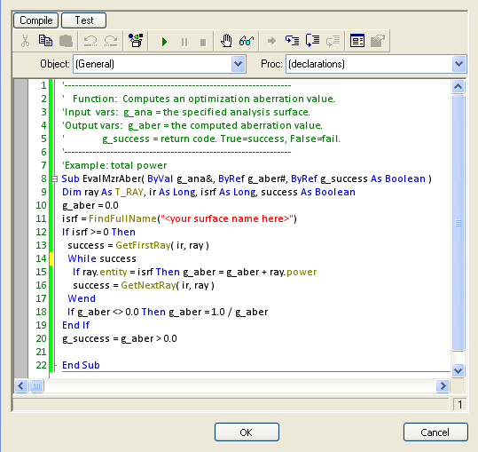
Moving next to the Merit Function Aberrations Tab, select the Aberration Definition type User scripted aberration. Select the Analysis Surface "Output Beam" as the Analysis Surface to Evaluate.  Right-click on the User scripted aberration entry and select the option "Edit user-defined script aberration" from the drop-down menu. The default dialog for this feature will appear as shown in Figure 3-4. Note that FRED provides one input value to the routine; g_ana (of type Long), the node number of the Analysis Surface designated in the Analysis Surface to Evaluate entry. The routine provides for two output values; g_aber (of type Double), the value of the computed merit function aberration, and g_success (of type Boolean), a return code signaling success or failure of the merit function computation. The example provided by default is a computation designed to maximize total power on a specified surface. Here, a loop over all rays is executed and the variable g_aber is used as an accumulator. Maximization of the power is achieved by minimizing the inverse of g_aber. Note that the routine returns True for g_success only if g_aber is greater than zero which is an indirect way of insuring that at least one ray has ended on the surface.

Figure 3-4. Default User-defined scripted merit function editor dialog.

Our objective in using the User scripted aberration merit function Type will be to determine the best focus z-position of all rays exiting the afocal and force this to a large value.  Since the Analysis Surface "Output Beam" is "attached" to the second surface of the second lens, its Reference Coordinate System is that of the same surface, namely "Afocal.SLB-20-60P (011-1360) OS.Surf 2". This is also the surface on which the rays are located. Therefore, the name of the parent coordinate system for the Analysis Surface (determined on line 12 from the T_OPERATION structure) can also serve as the first argument of the script command BestFocus (line 14) which serves as a filter for rays to be used in the calculation. By setting g_aber equal to the absolute value of 1/(z best focus) (line 15), the minimization process of the optimization routine will naturally force best focus towards infinity. Finalize the merit function definition by pressing the "Compile" button to insure there are no syntax errors. The functionality of the routine can also be tested by pressing the "Test" button which opens the dialog shown in Figure 3-6. Checking the box Trace rays before performing the test option followed by pressing the "Test" button causes FRED to execute the user-defined merit function after tracing rays then returns the computed value for g_aber on the row entitled "Test results (computed value)" and the value for g_success for the "Test code".

'----------------------------------------------------------------

'   Function:  Computes an optimization aberration value.

'Input  vars:  g_ana = the specified analysis surface.

'Output vars:  g_aber = the computed aberration value.

'              g_success = return code. True=success, False=fail.

'----------------------------------------------------------------

'Collimated output

Sub EvalMzrAber( ByVal g_ana&, ByRef g_aber#, ByRef g_success As Boolean )

Dim bf As T_BESTFOCUS, op As T_OPERATION

'get position orientation operation #0 from the analysis surface

GetOperation g_ana, 0, op

'compute the best focus for rays on op.parent and store in the T_BESTFOCUS structure

BestFocus op.parent, -1, bf

'aberration value is the inverse of the z best focus position

g_aber = Abs(1/bf.z)

'success if we have gotten to this point

g_success = True

End Sub

Figure 3-5. User-defined merit function aberration script designed to force best focus toward infinity

Figure 3-6. User-defined scripted merit function test dialog.

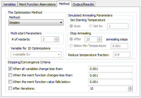
One final step is required before the optimization can be launched. Navigate to the Method tab in order to set the Optimization Method, and the Stopping/Convergence Criteria. See the optimization help topic for detailed information on these options. In this example, we want to use the Simplex method and allow the optimization to proceed until all of the variables have changed by less than 0.001. The Method tab should be configured as shown in Figure 3-7 below.

Figure 3-7. Method tab setup.

Lastly, we need to setup the Output/Results tab as shown in Figure 3-8.  Check the "Variables" box so that the value of the merit function and variables is printed to the output window on every iteration.

Figure 3-8. Method tab setup.

The optimization setup is now complete and ready for execution (hit Apply or OK on the dialog). From the Main Menu, Optimize select the option Optimize as indicated in Figure 3-9. FRED begins the optimization by performing a bracket search before proceeding with the minimization process. For more information on the Optimizer, consult FRED's Online Help. Results from the Output Window are shown in Figure 3-10 with the lens spacing quickly converging to a z-spacing of 41.45054 mm which corresponds to a best focus position of -23489.77313876 mm.

Figure 3-9. Launching FRED's Optimizer.

Figure 3-10. Optimizer data printed to Output Window.

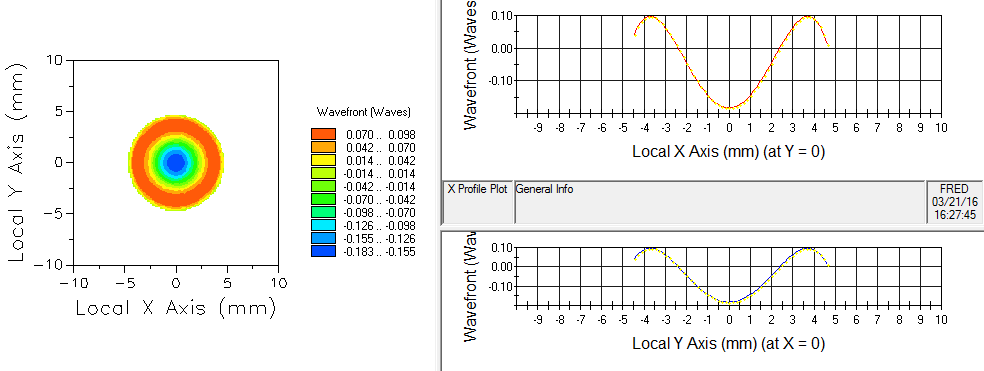
The new configuration can now be analyzed by running a raytrace, computing the Scalar Field at Analysis Surface "Output Beam" and plotting the wavefront as shown in Figure 3-11. Comparing this result with that of Figure 2-5 in the Intermediate tutorial section, the peak-to-valley wavefront error has been reduced from more than λ/2 to less than λ/4.

Figure 3-11. Wavefront calculation at afocal output aperture after optimization for most negative best geometric focus.

Merit Function for Collimation: Minimization of Wavefront peak-to-valley

Construction of a merit function for minimization of wavefront peak-to-valley variation also requires the User scripted aberration Type. The process involves three basic steps: 1) computation of the scalar field at the Analysis Surface "Output Beam", 2) computation of the Wavefront based upon the real and imaginary parts of the scalar field, and 3) finding the minimum and maximum values of the wavefront in order to construct the merit function g_aber.

The script shown in Figure 3-12 accomplishes the basic steps outlined above.  In the first part of the script, the scalar field is calculated using the analysis surface referenced by variable g_ana, whose value corresponds to the node that is selected in the "Analysis Surface to Evaluate" parameter in the GUI.  The resulting scalar field data is stored in an Analysis Results Node, referenced by the variable "arn" in the script, and the wavefront data is then extracted from the "ARN" using the ARNComputeWavefront command.  At this point, the wavefront data is stored in the array variable, "wf()", and the minimum and maximum values should be retrieved from the data array.  A double loop over the wf() data array is performed and each cell value is checked to determine if it is the new minimum or maximum value.  Also note that a cell value of 1E+308 is the equivalent of a NaN in the data array and we exclude this value from the determination of the minimum and maximum.  Finally, the merit function aberration value, g_aber, is defined as the difference between the maximum and minimum values.

'----------------------------------------------------------------

'   Function:  Computes an optimization aberration value.

'Input  vars:  g_ana = the specified analysis surface.

'Output vars:  g_aber = the computed aberration value.

'              g_success = return code. True=success, False=fail.

'----------------------------------------------------------------

'Example: wavefront peak to valley

Sub EvalMzrAber( ByVal g_ana&, ByRef g_aber#, ByRef g_success As Boolean )

g_aber = 0.0

'Calculate Scalar Field, put the result in an ARN, extract the wavefront data array

Dim arn As Long

Dim wf() As Double

ScalarFieldToARN( g_ana, "Optimizer SF", arn )

ARNComputeWavefront( arn, wf() )

'Retrieve wavefront min and max by looping over data array.

'Note that the data array uses a value of 1E+308 as a NaN equivalent.

Dim i As Long, j As Long

Dim vmin As Double, vmax As Double, curval As Double

For i = 0 To UBound(wf,1)

    For j = 0 To UBound(wf,2)

        curval = wf(i,j)

        If curval < 1E308 Then

            'Check for new minimum value

            If curval < vmin Then

                vmin = curval

            End If

            'Check for new maximum value

            If curval > vmax Then

                vmax = curval

            End If

        End If       

    Next

Next

'Calculate the peak-to-valley

g_aber = vmax - vmin

'Success condition

g_success = g_aber > 0.0

End Sub

Figure 3-12. User-defined merit function for minimization of wavefront peak-to-valley.

This merit function aberration can simply be added to the list as a second row on the Merit Function Aberrations tab as shown in Figure 3-13. Note that each row is equipped with an "Active" check box which allows any combination of merit functions to be used. For the next optimization run, we activate only the newly defined wavefront peak-to-valley aberration.

Figure 3-13. Multiple merit function definitions. The "Active" check box allows various combinations of merit function to be used.

Running the optimization a second time using the merit function shown in Figure 3-12 leads to a change in lens spacing of  Δz~35 μm from 41.45054 mm to 41.48515 mm. The peak-to-valley wavefront error is reduced from ~λ/4 to ~λ/5.

Figure 3-14. Wavefront calculation at afocal output aperture after optimization for minimum peak-to-valley.

Down Range Beam Profile

It is now of interest to investigate the beam profile downrange from the afocal for the two configurations arrived at by the optimizer. Create a new Analysis Surface and give it the name "Downrange". Set the X & Y Min.Max values to +/-10 mm and the number of divisions to 121. Set the Scale factor to 2. Press to OK button then drag-and-drop this new Analysis Surface onto the afocal exit surface "Afocal.SLB-20-60P (011-1360) OS.Surf 2". Open the Analysis Surface dialog and append a new Location entry to shift the measurement plane to the output beam's Rayleigh range of approximately 80,000 mm. The new Analysis Surface dialog should be configured as shown in Figure 3-15.

Figure 3-15. New Analysis Surface for downrange beam profile calculations.

Figures 3-16 & 3-17 below show the beam profile for the two afocal configurations; largest z-distance for best geometric focus and minimum peak-to-valley wavefront, respectively.  Configuring the model for each case can be easily done by navigating to the Output/Results tab of the optimization dialog, right mouse clicking on one of the results (one row per optimization run) and selecting the, "Apply to Document", option.  You will then need to perform the raytrace and scalar field calculation.  Most notably, neither profile has retained the initial Gaussian shape of the input beam. This result can be attributed to spherical aberration introduced by both the plano-concave and plano-convex lenses. Also, the peak irradiance is approximately 35% higher for the second case where the wavefront peak-to-valley was minimized. This is the result of having moved energy residing in the ring structure of Figure 3-16 into the central region of the profile in Figure 3-17. The user is encouraged to examine the beam profiles at several distances beyond the Rayleigh range. Note that these calculations can be made by simply editing the Z-shift and Scale factor of the Analysis Surface "Downrange" and re-calculating the irradiance.

Figure 3-16. Beam profile at Rayleigh range for lens spacing 41.45054 mm.

Figure 3-17. Beam profile at Rayleigh range for lens spacing 41.48515 mm.

Further improvement of afocal performance can be achieved by converting the pure spherical surfaces of the concave and convex elements to standard aspheres (even terms only) thereby adding more degrees of freedom to the optimization process. This conversion process is illustrated in the movie clip Figure 3-18. Since FRED will not retain terms with zero coefficients, a small value (1E-20) has been added to the 4^th order term. Repeat this process for the convex surface of the second lens.

Figure 3-18. Conversion of the concave surface from Conicoid to Standard Asphere (Video).

Once these surfaces are converted to aspheres, their conic constants and 4th order coefficients can be added to the list of Optimization Variables. Note that both the conic constant and aspheric coefficients are included among the list of built-in variables on the Optimization Variables Tab under the heading "Type". Unlike the Position/Orientation Type, the Conic constant has no Index # or Subindex #. These entries should be left with their default values of -1. For both surfaces, this parameter will be allowed to vary between the values -1 and +1. With regard to the aspheric coefficients, FRED's Online Help shows that the 4th order aspheric coefficient for a Standard Asphere surface occupies Index # 2. The Lower and Upper limits on these values are dictated to some extent by the clear apertures of 5 and 10 on the concave and convex elements. Figure 3-19 shows these four entries added to the variables list. The "Current Value" column has been populated for each variable by highlighting the four new rows, right-clicking and selecting the option "Get Starting Value(s) from Doc".

Figure 3-19. Conic constants and 4th order aspheric coefficients added as optimization variables.

An optimization launched with these additional variables allows the peak-to-valley wavefront variation to be reduced to less than λ/1000 as evidenced by Figure 3-20, where the intrinsic aberration value (i.e. the PV wavefront) is indicated to be 0.00095. All variables remain within their prescribed limits.

Figure 3-20. Merit function and variable values after optimization.

A computation of the irradiance profile using the Analysis Surface "Downrange" located at the Rayleigh range is shown in Figure 3-21. This profile shows that the spherical aberration encountered with the simple concave-convex elements has been eliminated as evidenced by its Gaussian shape and the fact that the beam radius is √2 times that of the beam exiting the afocal aperture (4mm beam radius exiting the second lens). The reader can verify this by performing a normalization on the data (right-click, select Scale Data and choose the "Normalize max value to 1" option as shown in Figure 3-22) then measure the X-axis distance to where the amplitude drops to e^-2 (0.135) on the X Profile Plot.

Figure 3-21. Irradiance profile at Rayleigh range after five variable optimization for minimum wavefront error at exit aperture.

Figure 3-22. Normalizing chart data using the Scale Data option.

This concludes the Advanced section of the Laser Illuminator tutorial. The reader is encouraged to extend this process to configurations in which the input beam waist is not located at the afocal input aperture.