In the Basic level tutorial, users 1) learn the fundamentals of constructing geometry by adding catalog lenses to form an afocal telescope, 2) construct a simple laser source, and 3) perform analyses of the afocal output.

Note: The videos included in this tutorial are hosted by YouTube and an internet connection is required to view them.  Controls embedded into the video player will allow you to view the videos in full screen and/or change the video resolution.

Afocal Telescope from Catalog Lenses

Begin the Tutorial by opening a blank FRED document (File>New>Fred Type, keystroke Ctrl+N or Toolbar button  ). You should see the view shown below in Figure 1-1 within the FRED application window.

Figure 1-1. New FRED document.

This tutorial begins by constructing a simple Galilean afocal telescope from two catalog lenses. These lenses will be placed in a Subassembly named "Afocal" and comprised of a plano-concave lens (part # 015-0040) and a plano-convex lens (part # 011-1360) from the OptoSigma catalog separated by a distance 41.32mm.

Begin by inserting in the Geometry folder a Subassembly which will contain the lens elements listed above. The Subassembly is a convenient organizational entity. All entities created within a Subassembly inherit the coordinate system of the Subassembly and therefore move as a unit when linear transformations are applied to the Subassembly.

Create a new Subassembly by one of four methods:

1.From the Main Menu, Create > New Subassembly

2.Keystroke Ctrl+Alt+S

3.Create Toolbar button

4.Right-click on Geometry folder and select option Create New Subassembly

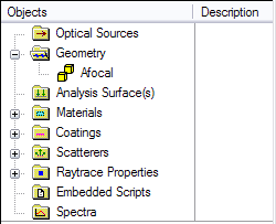
Name this entry "Afocal". The new Subassembly now appears in the Tree as shown in the Figure 1-2 below:

Figure 1-2. Afocal Subassembly entry in Geometry folder.

Enter the first lens by highlighting the "Afocal" subassembly then right-click to expose its drop-down menu. Selecting the option Insert Lens from Catalog near the bottom of the list causes the Select Lens from Catalog spreadsheet dialog to appear. From the Lens Catalog drop-down at the top, select the OptoSigma Corporation catalog then scroll to and highlight the first lens SLB-10-15N (015-0040) (f = -15mm) and hit the Apply button. This inserts the lens leaving the dialog box open. Note that this lens now appears as an entry in the Geometry folder under the Afocal subassembly. Next, scroll to and highlight the second lens SLB-20-60P (OS 011-1360) (f = 60mm) and hit the OK button to insert this lens and close the dialog. Note that both lenses now have an entry in the Geometry folder under the Afocal subassembly and appear in the 3D View with their vertices coincident at the origin of the Afocal subassembly coordinate system. The movie clip in Figure 1-3 shows the above process in action.

Figure 1-3. Adding afocal elements from Lens catalog (Video).

Best performance of the afocal dictates that the convex surface of the second lens be the exit surface. Changing the configuration can be done one of two ways: 1) apply a 180° rotation about the X or Y axis, or 2) reassign the radii s1s2 & s2s1. The latter is preferable since this maintains the original orientation of the lens coordinate system. Double-click on the SLB-20-60P (011-1360) OS Lens icon to open its dialog box, change the "Front radius" from 31.14 to zero and the "Back radius" from zero to -31.14 then hit the dialog OK button. The lenses now appear as shown in Figure 1-3.

Figure 1-4. Catalog lenses with second lens radii exchanged.

The lens spacing may now be set by placing the second lens (SLB-20-60P (011-1360) OS) in the coordinate system of the first lens (SLB-10-15N (015-0040) OS) then adding a z-shift of 41.32 mm stated above. This combination of lenses with this spacing results an afocal of magnification M=4. Right-click on the second lens icon and select the Position/Orientation option. Use the Entity Picker to select the Reference coordinate system of the back surface of the second lens "Afocal.SLB-10-15N (015-0040) OS.Surface 2". Next, append a shift command and enter the aforementioned spacing distance. The movie clip in Figure 1-5 demonstrates this re-parenting and shifting operation.

Figure 1-5. Relative referencing and positioning of second lens (Video).

Coherent Source: Gaussian Beam

With the lenses now properly in place, the next step is the addition of our source representing a laser beam. The Laser Beam (00 mode) type Source Primitive represents a TEM₀₀ Gaussian beam with its beam waist at the source location.

A Laser Beam (00 mode) source type is added by one of the following methods:

1.From the Main Menu, Create > Source Primitive > Laser Beam (00 mode)

2.Right-click on Optical Sources folder and select option Create New Source Primitive > Laser Beam (00 mode)

3.Create Toolbar button:

In the resulting dialog, set the Power (watts) to 1.0 (parameter 0), specify 1/e2 beam semi-width of 1 mm (parameter 2), and set the semi-aperture of the source grid to 2 mm (parameter 3).  The number of sample points across the grid diameter should be 21 (parameter 1). This definition means that a circular grid of 21x21 rays across a +/-2 mm source aperture has its rays apodized (weighted) to produce a Gaussian beam with a 1 mm 1/e² half width.

In the wavelength attributes section, use the "Single" option and set the wavelength to 0.6328 microns.  Set the "Source Draw Color" to be red.

In the Location/Orientation portion of the dialog, place the source in the Reference Coordinate System of the Afocal subassembly with a z-shift of -2 mm. The resulting source dialog should appear as in Figure 1-6.

Figure 1-6. Laser Beam (00 mode) source dialog defining a TEM₀₀ Gaussian beam at λ = 0.6328 μm.

As with all coherent sources regardless of type, each ray in the grid is represented as a Gaussian beamlet whose waist size is determined largely by the spacing between adjacent rays. In the specific case of the Laser Beam (00 mode) type Source Primitive, the amplitudes of the Gaussian beamlets are apodized such that their coherent sum results in a single TEM₀₀ Gaussian beam. These characteristics can be observed by first creating an Analysis Surface.  The Analysis Surface provides a user-defined planar grid on which various calculations are made. An Analysis Surface is created by one of three methods:

1.From the Main Menu, Create>New Analysis Surface

2.Keystroke Ctrl+Alt+N

3.Analysis Toolbar button

From the default Analysis Surface dialog box, change its name to Irradiance at laser source, set the scale factor to 1.5 and the number of pixels in X & Y to 101. "Attach" this Analysis Surface directly to the source using the method of drag-and-drop. The movie clip in Figure 1-7 shows these steps.

Figure 1-7. Adding an Analysis Surface for examination of laser source before propagation (Video).

The source at its origination plane can be examined by simply creating the rays without tracing. Create the rays without tracing using one of three methods:

1.From the Main menu, Raytrace>Create All Sources

2.Keystroke Ctrl+Shft+F8

3.Raytrace Toolbar button

Let us now use the Analysis tool Ray Summary to examine these newly created ray. The Ray Summary prints to the Output Window a listing of Ray Count, Total Incoherent Power and the Name . Entries under the heading Name indicate which entity the rays are currently associated.

The Ray Summary is invoked by one of three methods:

1.From the Main Menu, Analyses>Ray Summary

2.Keystroke Shft+F11

3.Analysis Toolbar button

Press OK on the resulting dialog to perform the Ray Summary analysis for All Rays in the system.

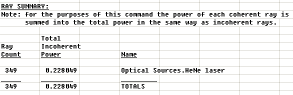
Figure 1-8. Ray Summary after ray creation but before tracing.

Figure 1-8 shows the Output Window after executing the Ray Summary before tracing. In this case, the rays are associated with the HeNe source since they have been created but not yet traced. Next, note that the Total Incoherent Power differs significantly from the power assigned to the source in Figure 1-6. The discrepancy stems from the fact that the Ray Summary always returns the Incoherent Power. Evaluation of the incoherent power for a coherent source ignores the cross-term (constructive/destructive interference) associated with coherent summation of the beamlets. For example, consider two beamlets represented by scalar field E_i = E_ie^iφ but with different phases φ1 and φ2. The irradiance due to these two beamlets is then

                              I_tot = EE^* = (E₁ + E₂)(E₁^* + E₂^*) = E₁E₁^* + E₂E₂^* + E₁E₂^*e^i(φ1-φ2) +E₁^*E₂e^-i(φ1-φ2) 

If, for simplicity we let E₁ = E₂, then

                              I_tot = 2I₁ + 2I₁cos(φ1-φ2)

If the two beams are incoherent then phase is irrelevant and the cosine term is of no consequence yielding I_tot = 2I₁. If, however, the beams are coherent then their total irradiance can vary between 0 [φ1-φ2=(2m+1)π] and 4I₁ [φ1-φ2=2mπ] depending upon their relative phase difference. Since P = ∫_A I dA, the total power obeys the same basic relation. Therefore, the total power of a coherent source can be correctly evaluated only by computing irradiance. The power value returned by the Ray Summary is not valid for coherent rays.

With this in mind, we now compute the irradiance of the source. An Irradiance Spread Function calculation is invoked using one of the following methods:

1.From the Main Menu, Analyses>Irradiance Spread Function

2.Keystroke Ctrl+F10

3.Analysis Toolbar button

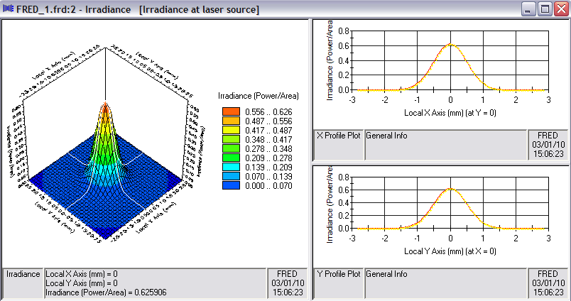
Figure 1-9 below shows the resulting irradiance calculation at the source creation plane using the Analysis Surface "attached" as in Figure 1-7. FRED's Chart Viewer displays the irradiance in three panes; a three-dimensional perspective chart on the left and two orthogonal profiles displayed on the right.

Figure 1-9. Irradiance at source location before tracing.

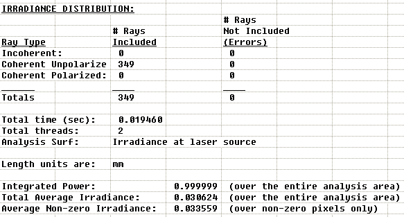
Figure 1-10 below shows a section of the Output Window associated with the irradiance calculation.

Figure 1-10. Data output from irradiance calculation.

Note that the Integrated Power is, in fact, 1 as assigned in Figure 1-6. The peak irradiance is (2/πω²)~0.63, which has units W/mm² in this case since the document system units are millimeters.

Tracing Rays and Examining Afocal Output

We are now in position to trace the source rays through the afocal. While there are numerous options for raytracing in FRED, we restrict ourselves at this stage to a basic raytrace initiated by one of three methods:

1.From the Main menu, Raytrace > Trace and Render or Raytrace>Trace All Sources

2.Keystroke Ctrl+Shft+F7 or Ctrl+Shft+F5

3.Raytrace Toolbar button  or 

The Trace and Render option creates rays according to the source definition and performs the trace drawing each ray's trajectory in the 3D View. The Trace All Sources option creates rays according to the source definition and performs the trace without drawing the ray trajectories. The difference between drawing and not drawing the ray trajectories carries two important consequences:

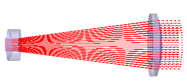
Using the Trace and Render option, trace the source rays through the afocal as shown in Figure 1-11 below. Note that the rays exit the second lens as dashed lines indicating that there are no further surface intersections.

Figure 1-11. Raytrace through afocal.

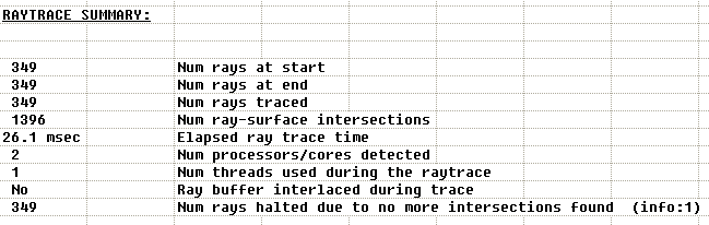
Each time a raytrace is executed, FRED prints a Raytrace Summary (see Figure 1-12) to the Output Window. The Raytrace Summary details the number of rays at start, number of rays at end, number of rays traced, number of surface intersections, elapse trace time, number of processors detected, number of threads used during the trace, whether buffer interlacing occurred during the trace, and any Warning/Error/Information messages. Note from 2) above that Trace and Render has forced the use of only one thread (CPU).

Figure 1-12. Raytrace Summary printed at conclusion of raytrace.

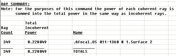
Let us again examine the Ray Summary after the raytrace. Figure 1-13 below shows that the rays are now "associated with" or "on" Surface 2 of the second lens. A key point to understand is that at the end of the raytrace, any given ray can be associated with only one entity in the model.  This association happens either when the ray is totally absorbed by an entity or when no further intersections can be found after leaving the entity. Here, the term "entity" refers to either a source or a surface thereby including the case encountered earlier when rays were created and evaluated at the source as in Figure 1-8.

Figure 1-13. Output from the Ray Summary Analysis option.

With rays now "on" surface 2 of the second lens, create another Analysis Surface and give it the name "Output Beam". Uncheck the Autoscale option, set Xmin=-10 & Xmax=10, set the Divisions in each direction to 121 and hit the OK button.  "Attach" this Analysis Surface to Surface 2 of the second lens using the drag-and-drop method demonstrated in Figure 1-6. This new Analysis Surface Location should now be in the Reference Coordinate System of "Afocal.SLB-20-60P (011-1360) OS.Surface 2" and have the Ray Specification Rays on Surface "Geometry.Afocal.SLB-20-60P (011-1360) OS.Surface 2" as shown below in Figure 1-14.

Figure 1-14. Analysis Surface dialog "attached" to Surface 2 of second lens.

Using the "Output Beam" Analysis Surface, perform an Irradiance calculation using the Irradiance Spread Function as described previous to Figure 1-9 above. When the Irradiance calculation is requested, note that a dialog appears listing all currently existing Analysis Surfaces as shown in Figure 1-15 below. It will now be necessary to select the "Output Beam" Analysis Surface from List of Available Analysis Surfaces before clicking the OK button. The Analysis Surface "Irradiance at laser source" with the Ray Specification Rays on surface "Optical Sources.HeNe laser" can't be used here since we know from the Ray Summary output of Figure 1-13 that the rays are no longer on the source.

Figure 1-15. Analysis Surface selection dialog.

To confirm the magnification of 4 has been achieved, right-click in the Chart and select the option Scale Data from the drop-down menu. Normalize the data to unity by selecting the first option in the dialog. Using the mouse in the X Profile Plot, slide the cursor horizontally such that the irradiance reading is approximately 0.135. This is the amplitude of a unit irradiance Gaussian beam at its 1/e² half-width. Note the Local X-value is 4mm thus confirming that the 1mm radius input beam has been expanded by a factor of four. The movie clip in Figure 1-16 shows this process in action.

Figure 1-16. Measurement of beam radius from irradiance at output of afocal (Video).

This concludes the Basic Tutorial. Save the system as a FRED document before proceeding to the Intermediate Tutorial.