The goal of this tutorial is to provide new users with an introduction to the basics of the FRED interface through construction of a simple two element Galilean beam expander.
The following items are covered in this tutorial:
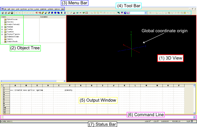
Introduction to the Graphical User Interface FRED has a multiple document interface, which means that you can have many different files open simultaneously. Create a new document in FRED by going to Menu > File > New > Fred Type. The graphical interface of a FRED document is grouped into seven unique components: 1. 3D View The 3D View is updated in real time as components are added to the model and can be interactively manipulated with the mouse and keyboard. 2. Object Tree The Object Tree is an organizational structure that allows construction of objects, sources and optical properties as well as property assignments. Each object type is stored in the appropriate folder of the object tree and each folder can be expanded to show the objects that are contained within it. As objects are added to the model, the object tree is updated automatically. 3. Menu Bar The Menu Bar is a generic way to access any of FRED's features (file operations, object creation, analyses functions, etc). If the user is unsure where/how to access a function, the Menu Bar is a likely place to look. 4. Tool Bar The Tool Bar can be customized to contain buttons which provide quick access to commonly used functions. 5. Output Window The Output Window displays information to the user whenever an action is performed. For example, statistical information is printed to the output window at the end of analyses and raytraces. The Output Window should always be checked for informative messages, since this will indicate any potential errors and provide insight for debugging and verifying system models. (TIP: Navigate to Menu > View > Output Window and toggle the "Cells" option to view the output window as a spreadsheet) 6. Command Line The Command Line allows entry of any of FRED's scripting commands. For anything more complicated than a single command, it is best to use the script editor (not discussed in this tutorial). 7. Status Bar The Status Bar contains basic information about the current FRED document, including system and wavelength units.
The Preferences dialog allows for customization between FRED sessions and can be opened by navigating to Menu > Tools > Preferences. Preference configuration is important for maximizing the performance of FRED for a given PC. For more information on Preference optimization, please see this Knowledge Base article: Preference Optimization.
The Tool Bar menu can also be customized. To add buttons to the toolbar, navigate to Menu > View > Toolbars and click on "Customize". In the resulting dialog, select a category and drag the desired button icon from the dialog up to the Tool Bar using the mouse. The toolbar buttons can be handy if you find yourself creating certain objects or performing certain analyses regularly.
The 3D View window is updated when new objects are added to the model and the user can interactively rotate, zoom, pan and select objects directly from the 3D View window using their mouse and keyboard. It is important to note that use user may need to "resize" the 3D view when objects are added to the document so that the entire system can be viewed with the proper scaling. The "view all" toolbar button,
The 3D View menu bar item offers a list of options specific to the 3D View. Most importantly there are three modes for operating within the 3D View; Trackball, Magnify, and Object Selection. Each mode interprets the keyboard and mouse controls in a different manner, with Trackball mode being the most common.
The following controls allow manipulation of the 3D view, with the operation mode indicated in parenthesis: Rotation (Trackball) Click and hold the left mouse button in the 3D View window and rotate by moving the mouse. Pan (Trackball) Hold Ctrl and the center mouse button while moving the mouse. Zoom (Trackball) Scroll up and down with the mouse wheel to zoom in and out. Set Object as Center of Rotation (Trackball) Left click on object in the 3D View and then press the Space bar on the keyboard. Select Object(s) on Object Tree (Object Selection) Left mouse click and hold in the 3D view to draw a selection rectangle. All objects within this rectangle are selected and highlighted on the object tree. Magnify Region (Magnify) Left mouse click and hold in the 3D view to draw a rectangular region of the 3D view to be magnified. Demagnify Region (Magnify) Shift + Left mouse click and hold in the 3D view to draw a rectangular region of the 3D view to be demagnified.
FRED has several different geometry types which can be added to the Geometry folder on the object tree. These different geometry types are summarized below:
Geometry can be added to the FRED document in one of two ways: •Right mouse click on the Geometry folder on the object tree and choose "Create...." •Navigate to Menu > Create > "New..."
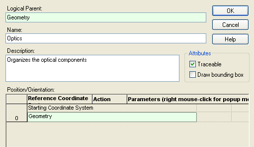
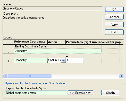
Start the construction of the simple beam expander by adding a new subassembly to the Geometry folder on the object tree. The subassembly is added first so that the optical components can be organized together and a unit on the object tree. •Right mouse click on the Geometry folder on the object tree and choose "Create New Subassembly" from the context menu. •Name the subassembly node "Optics". •Give the subassembly node the description "Organizes the optical components". •Click "OK" to accept the settings and close the dialog box.
After adding the subassembly you will see that the Geometry folder on the object tree now has a "+" symbol next to it. Click on the "+" symbol to expand out the Geometry folder and reveal the newly added "Optics" subassembly node. In this system, the subassembly node is referred to as a child of the Geometry folder. In turn, the Geometry folder is referred to as the parent of the subassembly. More details on this hierarchy will be discussed later, but it is sufficient to say now that new geometry is created as a child node to whatever object was currently selected at the time of its creation.
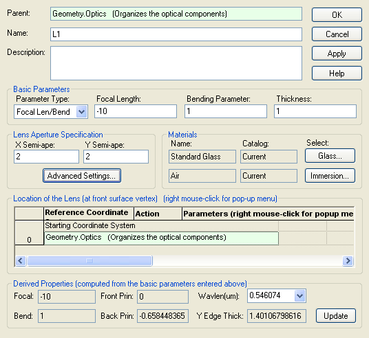
The lens elements for the beam expander will have the following properties:
Create the first lens by right mouse clicking on the "Optics" subassembly node and selecting "Create New Lens" from the context menu. Enter the parameters for lens "L1" into the lens dialog and hit "OK" to accept the settings. Note that the "Optics" subassembly node now contains a child lens node named "L1". You can always double mouse click on an entity on the object tree to re-open that entity's dialog for editing.
As mentioned in the section Manipulating the 3D View, it may be necessary to re-size the 3D view using the "View All" toolbar button (
Create the second lens by right mouse clicking on the "Optics" subassembly node in the object tree and selecting "Create New Lens" from the context menu. Notice in the middle of the lens dialog that there is a section called "Location of the Lens (at front surface vertex)". This section of the dialog is used to control the position and orientation of the lens element. Entry #0 is the starting coordinate system for the lens element. In FRED, any object is allowed to be positioned relative to any other object. This is a very powerful feature because the user only has to know how objects are positioned relative to some reference, rather than knowing the explicit global coordinates. Additionally, it means that the user can move entire groups of objects at once while maintaining their relative configuration.
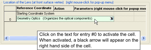
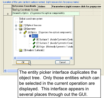
Change L2's starting coordinate system from the "Optics" subassembly to "L1" by mouse clicking on the text "Geometry.Optics (Organizes the optical components)" to activate the cell. Notice that there is now a black arrow on the right side of the cell. Click on the black arrow to activate what is called the Entity Picker Tool and then choose the "[5] L1" node from the interface and hit "OK". Entry #0 for the L2 node should now read "Geometry.Optics.L1". These steps are clarified in the images below.
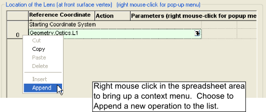
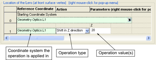
Now add the Z-shift to lens "L2". Right mouse click in the spreadsheet area of the operations list and choose "Append" from the context menu. The new row (operation #1) defaults to a "Shift" type operation with five columns. The first column is the coordinate system in which the operation will be performed, which can be selected using the entity picker interface. The second column sets the operation type, which can be selected from the drop-down list. The number and meaning of the remaining columns will depend on the type of operation that was selected. Using the drop-down list, set the operation type to "Shift in Z direction" and enter a value of 20. After hitting the "Apply" button on the lens dialog the 3D view is automatically updated.
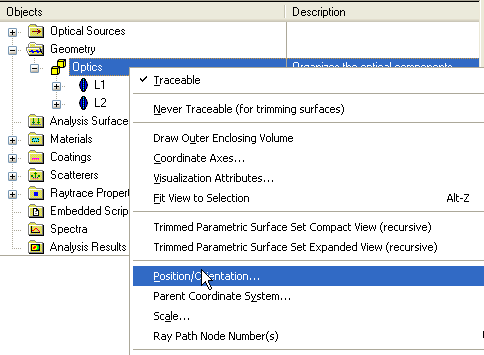
For the final step, shift the entire "Optics" subassembly 5 units along +Z. Right mouse click on the "Optics" subassembly node on the object tree and select "Position/Orientation" from the context menu. The position orientation dialog's functionality is identical to the embedded versions discussed earlier in the lens dialogs. Right mouse click in the spreadsheet area and choose "Append" to add another operation to the list. Set the new operation's type to "Shift in Z direction" and enter a value of 5. Hit "OK" and notice that the 3D view is updated. It is also important to note that L1 and L2 were shifted with the subassembly (remember, they are linked together) but have maintained their relative positioning with respect to each other.
Having constructed and positioned the geometry components, we will briefly divert to discuss the construction of FRED's object tree.
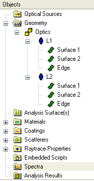
Object Tree Hierarchy and Organization At this point in the tutorial, the object tree in the FRED model should look like the following:
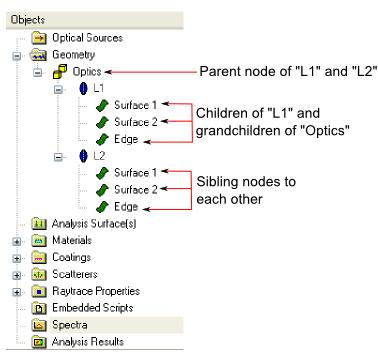
Each entity on the object tree is referred to as a node. The indentation structure of the tree indicates parent/child relationships. For example, L1 is a child node of the Optics subassembly. Conversely, the Optics subassembly is a parent node of both L1 and L2. Going one level further, the base surfaces of L1 (Surface 1, Surface 2 and Edge) are grandchild nodes of the Optics subassembly. Following this convention, the surfaces Surface 1, Surface 2 and Edge of lens node L1 are siblings. These relationships are diagrammed below for clarification.
Although there are surfaces with duplicate names on this object tree (Surface 1, Surface 2 and Edge), each surface occupies a unique space in the hierarchy and therefore has a unique full name. For example, Surface 1 of L1 has the unique full name "Geometry.Optics.L1.Surface 1". Similarly, Surface 2 of L2 has the unique full name "Geometry.Optics.L2.Surface 2". How is this full name constructed? Start at the parent folder on the object tree and move down through the hierarchy, appending the name of each node until you reach the desired entity. In our example of Surface 1, the flow is Geometry > Optics > L1 > Surface 1 to construct "Geometry.Optics.L1.Surface 1". If you look back at the entity picker tool dialog, you will recall that the coordinate system was referenced using the entity's full name.
Optical and mechanical properties such as materials, coatings and raytrace properties are ultimately assigned at the surface level (after all, this is what the rays intersect during the raytrace). There are two generic ways to assign properties to surfaces.
•Double mouse click on the surface's node on the object tree and use the corresponding tab in the dialog (Materials, Coating/Ray Control) •Drag and drop of the property from the corresponding property's folder up to a geometry node directly on the object tree
The first method is appropriate for assigning specific properties to an individual surface. However, it is more often the case that the user wishes to assign properties to a group of surfaces simultaneously. The drag and drop method will be discussed in this section of the tutorial.
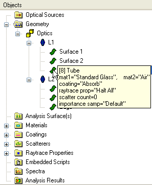
A tooltip will be displayed if you hover your mouse over an objects icon on the object tree, as shown in the image below. This tooltip is the quickest way to view the properties currently assigned to that object.
In the image above, the tooltip displays that the surface "Geometry.Optics.L1.Edge" has the following properties: •Node # = 8 (primarily used for scripting access) •Surface type = Tube •Materials assigned = Standard Glass and Air •Coating assigned = Absorb •Raytrace property = Halt All •Number of scatter models assigned = 0 •Number of importance samples assigned = 1 ("Default")
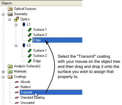
Rather than have the Edge surface's coating be "Absorb", make the coating be "Transmit". To do this, select the "Transmit" coating in the Coatings folder on the object tree and drag it up to the Edge surface node. You must have the object tree expanded out so that both the coating node and the surface node are visible.
After assigning the coating by drag and drop, verify that the property has been applied by hovering over the surface node's icon with the mouse and inspecting the tooltip. The tooltip should now display "coating='Transmit'".
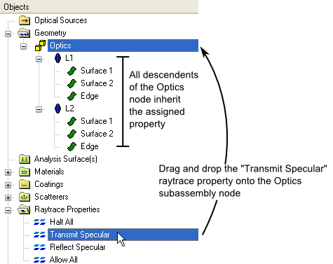
The drag and drop assignment method can not only be applied to an individual surface, it can use the object tree's hierarchy structure to assign properties to multiple surfaces at once. For example, assign the "Transmit Specular" raytrace property to the "Optics" subassembly node. Using the tree's hierarchy, every node which is a descendant (child, grandchild, etc.) of the Optics subassembly inherits the property being assigned.
Sources can be created in the following ways: •Right mouse click on the Optical Sources folder on the object tree and choose "Create...." •Navigate to Menu > Create > "New..."
There are three types of sources in FRED: Detailed Optical Source Used to construct a custom source by specifying ray starting positions, directions, coherence and power profiles. This is the source type which gives the user complete control over the source model. Source from IES File Creates a volume source from an IES file in ANSI/IESNA LM-63-2002 format. Source Primitives Used to quickly create a variety of common source types, including plane waves, point sources, diodes, rayfile sources, solar sources, etc.
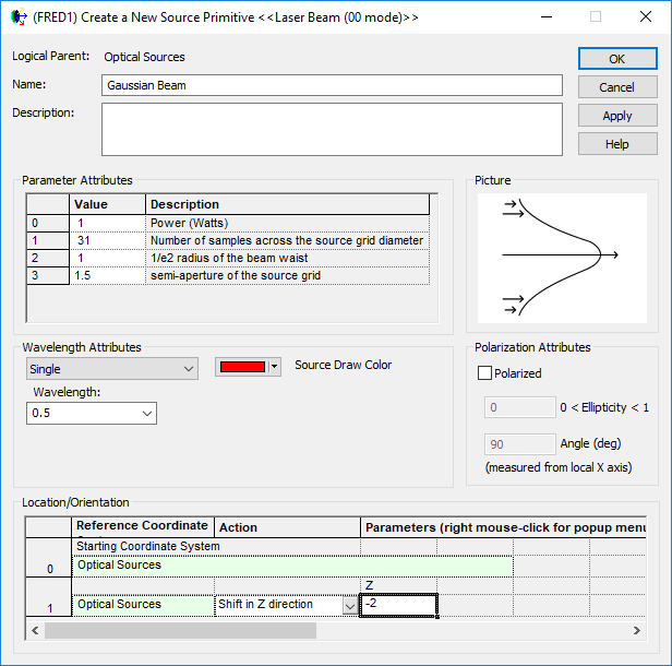
In this tutorial, a Laser Beam (00 mode) type Source Primitiveis going to be created as the input to the beam expander. Right mouse click on the Optical Sources folder and select "Create New Source Primitive" from the context menu and then choose "Laser Beam (00 mode)" from the sub-menu. Use the following settings for the source: Name: "GaussianBeam" Power: 1.0 Number of samples...: 31 1/e2 waist radius: 1.0 Grid semi-aperture: 1.5 Wavelength: Single, 0.5 microns Source Draw Color: Red Position: -2 along Z, relative to the first surface of L1
For clarification, the completed dialog is shown below.
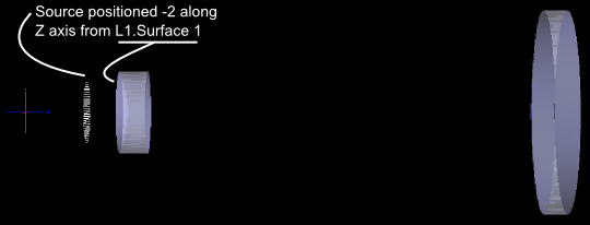
After hitting "OK" on the source dialog, you should verify in the 3D view that the source appears in the desired location. The current 3D view is shown below.
Analysis Surfaces are grids in space which define a sampled region over which to perform an analysis. Analysis Surfaces do not interact with rays during the raytrace, so they can be added to the document and modified at any time without the need to re-trace the geometry. The following methods can be used to create an analysis surface: •Right mouse click on the Analysis Surface(s) folder and select "New Analysis Surface" from the context menu •Menu > Create > New Analysis Surface
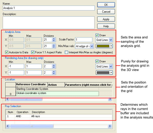
There are several sections of the analysis surface dialog which must be visited in order to ensure that the expected results are displayed. Each section of the default analysis dialog is briefly described in the following image:
Analysis Area Although the default option for defining the analysis area uses "Autosize to Data", this is almost never recommended. This option calculates the geometrical extent of the rays included in the analysis and sets the size of the grid to enclose those extents. It is recommended that the user manually set the X and Y Min/Max extents for the analysis area to ensure predictable results. Also note that because the autosize feature is geometrical, the results are likely not appropriate for coherent analysis since the field dimensions can be much different than the ray extents.
The number of divisions sets the sampling of the analysis area. Incoherent rays are "bucket counted" within a cell area. The larger the number of divisions in the analysis area the more rays will need to be traced to ensure that each pixel gets a reasonable ray count. For coherent calculations, a larger number of divisions may be used so that the field profile can be adequately sampled. A typical coherent calculation may use 101 x 101 pixels on a square grid.
Rendering Area If the number of divisions in the analysis area is significant, the user may not wish to draw the full sampling grid to the 3D view. Alternatively, the user can set a grid in the rendering area section of the dialog which is used solely for the purposes of drawing in the 3D view. This has no impact on the calculation performed.
Location This sets the position and orientation of the analysis grid in the model using the same controls as used for geometry and sources. The analysis is performed in the spatial location of the analysis grid.
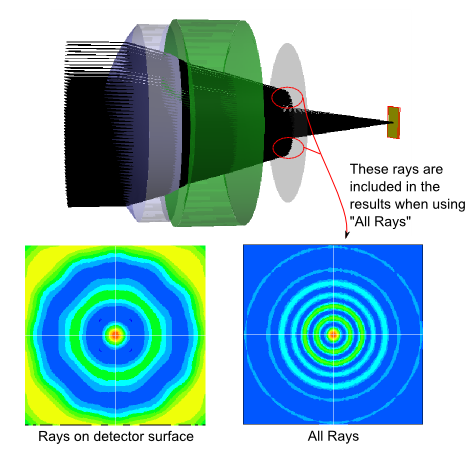
Ray Selection The ray selection is critical in setting up a proper analysis. Internally, each ray is "associated" with a source or surface in the model. This ray's association is with the last entity that ray intersected during the raytrace. At the completion of a non-sequential raytrace, rays can be associated with virtually any entity in the model and the user must define which subset of these rays are to be included in the analysis results. Consider the default ray selection criteria: AND All rays This criteria literally means that all rays (regardless of their current location) should be included in the analysis results. Any rays which are not stopped at the position of the analysis grid will be propagated free space along their current trajectory to intersect the analysis grid. Consider the following system which focuses a beam down through a clipping aperture to a detector plane. The analysis plane is located at the detector plane and the irradiance distributions are shown for two different ray selection criteria; only rays on the detector surface (left) and the default All Rays (right). The distribution shown on the right for the All Rays ray selection criteria includes the contribution at the detector plane from those rays which are halted at the aperture plane. The distribution on the left, which filters only rays on the detector surface, shows the effect of the aperture.
Add an analysis surface to the beam expander model by right mouse clicking on the Analysis Surface(s) folder on the object tree and selecting "New Analysis Surface" from the context menu.
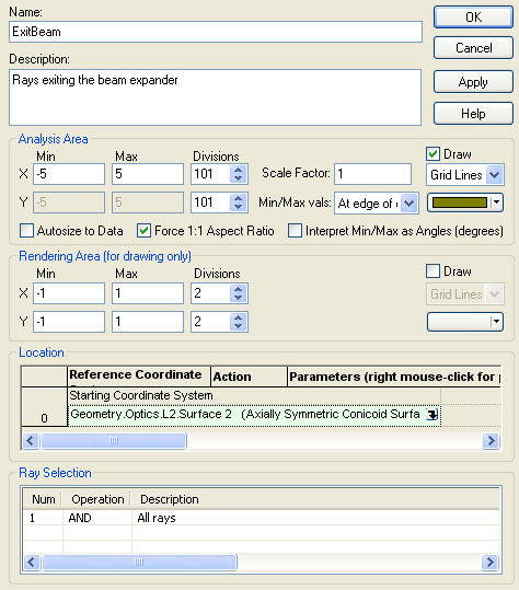
Enter the following parameters into the analysis surface dialog and press "OK" to accept the settings and add the analysis surface to the document:
Name = ExitBeam Description = Rays exiting the beam expander Analysis Area X Min = -5 Analysis Area X Max = 5 Divisions (X and Y) = 101 Rendering Area Draw = False Location = Coincident with "Geometry.Optics.L2.Surface 2"
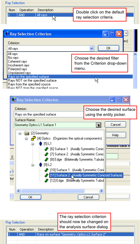
There are two ways to set the ray selection criteria for an analysis surface, manually within the analysis surface dialog or by drag and drop on the object tree. The following steps can be taken to manually change the ray selection criteria from the default "AND All rays" to a filter which only include rays that are associated with the specific surface.
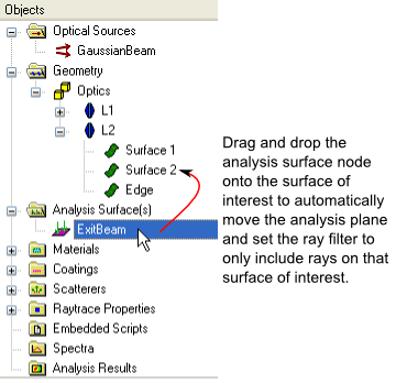
Alternatively, the analysis surface can be dragged and dropped from the Analysis Surface(s) folder on the object tree directly to the surface of interest. This will automatically position the analysis surface coincident with the surface and set the ray selection criteria to include only rays on that surface.
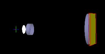
After creating and setting up the analysis surface, the beam expander system should look like the following image.
There are two basic raytrace types, raytrace with render and raytrace without render. The raytrace with render can be accessed in the following ways: •Menu > Raytrace > Trace and Render •Toolbar button:
The raytrace without render can be accessed in the following ways: •Menu > Raytrace > Trace All Sources •Toolbar button:
Why wouldn't you want to raytrace without rendering? One advantage of using FRED is that its raytracing and most analysis routines are multi-threaded to take advantage of all CPU cores on your computer. The Trace and Render functionality forces the raytrace to use only one thread. So, while the user gains insight into how the raytrace progresses through the system, there is also a speed penalty incurred compared to raytracing without rendering. The Trace All Sources function takes full advantage of the computer's processing power but does not provide any visual feedback to the user.
Most often, the Trace and Render function is used during the preliminary phases of modeling and the user switches to the Trace All Sources function once a larger number of rays are required for analysis. In this beam expander system, only a relatively small number of rays are being traced so there is no significant penalty for using the single-threaded Trace and Render functionality.
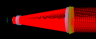
Perform a Trace and Render on the beam expander system.
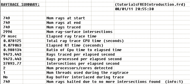
Regardless of the type of raytrace performed, the user should always check FRED's output window for status messages regarding how the raytrace proceeded. The raytrace output for the beam expander model is shown below.
FRED has a variety of analyses routines for looking at coherent and incoherent fields. Some of these analyses are: Positions Spot Diagram - X,Y ray intercept plot Polarization Spot Diagram - X,Y ray intercept and polarization ellipses plot Irradiance Spread Function - Power/Area Illuminance - Photometric Power/Area Coherent Scalar Field - Unpolarized coherent field analysis Coherent Vector Field - Polarized coherent field analysis Color Image - x,y chromaticity coordinates
Analysis routines can be performed in the following ways: •Menu > Analyses > (Select desired analysis) •Toolbar buttons ( •Keyboard Shortcuts (ex., Ctrl + F10 )
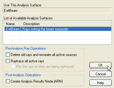
In this example beam expander the Irradiance Spread Function will be performed on rays exiting the second lens element using the "ExitBeam" analysis surface previously defined. After tracing the rays, perform the Irradiance Spread Function analysis by going to Menu > Analyses > Irradiance Spread Function. The user will be prompted by a dialog with several options:
List of Available Analysis Surfaces - If the model has more than one analysis surface the user must specify which to use Delete old rays and recreate all active sources - If the user wishes to re-create the sources rather than using the existing rays in the buffer Raytrace all active rays - If the user wishes to trace the current rays in the buffer before performing the analysis Plot the rays as they are being raytraced - If the user chooses to raytrace active rays and also wishes to see them drawn to the 3D view Create Analysis Results Node (ARN) - Creates a node in the Analysis Results folder on the object tree that stores the results of the analysis being performed for later review in the FRED session
The rays have already been traced in the previous section of this tutorial, therefore do not check any options on the analysis dialog and press "OK" to perform the analysis.
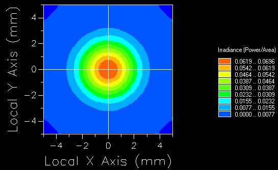
Once the analysis has finished, the results will be displayed in FRED's chart viewer in 3D and profiles. Right mouse clicking in the chart viewer will bring up a context menu for manipulating the data and specifying chart settings. The following image shows the irradiance spread function results with perspective view off.
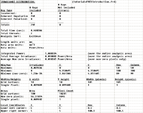
FRED's output window is extremely valuable for conveying information to the user regarding the most recently requested function. The user should always check the output window after performing a function for further insight in to model behavior and results. Consider the irradiance spread function that was performed in the previous section of this tutorial. At the conclusion of the analysis, the following information was printed to the output window:
Among the information printed to the output window is the number of rays included/excluded from the analysis, the total integrated power over the analysis surface area, the dimensions of the analysis surface area and pixels, and unit information.
|