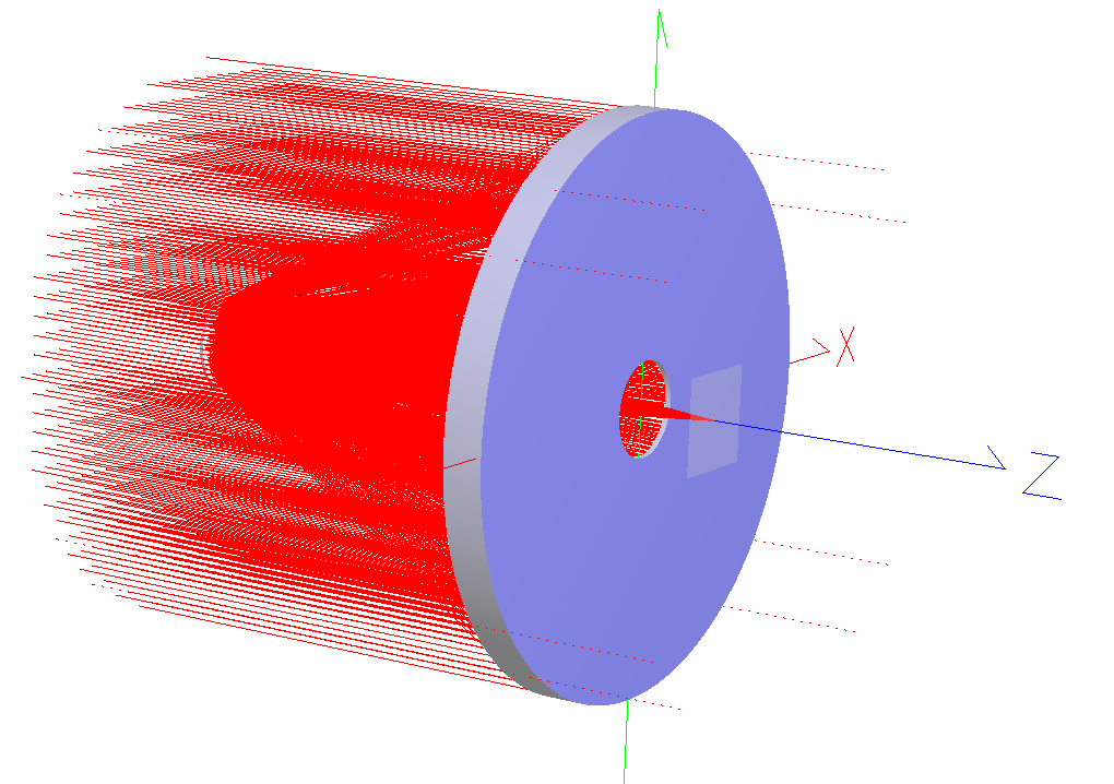
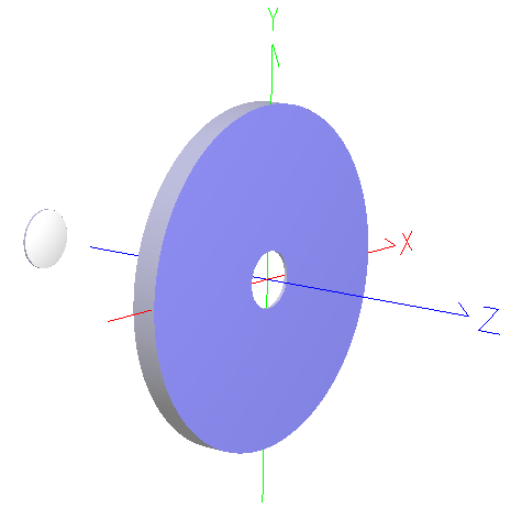
In this tutorial we will discuss how to build a simple Cassegrain telescope model from scratch in FRED without assuming any prior experience with the software. After this tutorial you will be able to create objects, apply properties, and perform raytracing and analyses. An image of the system to be constructed is shown below.
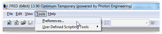
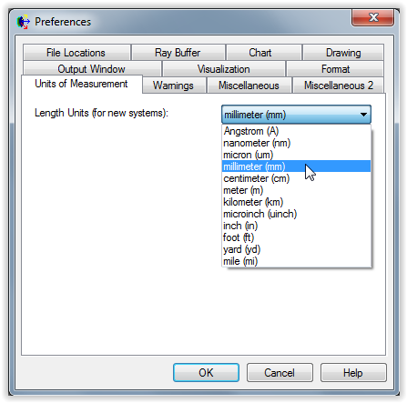
Before we start constructing the Cassegrain telescope model, we will want to setup some FRED preferences. While many preference settings can be adjusted dynamically while working on a FRED document, some preferences, such as units, must be changed before you create a FRED document. Upon starting your copy of FRED, navigate to Menu > Tools > Preferences.
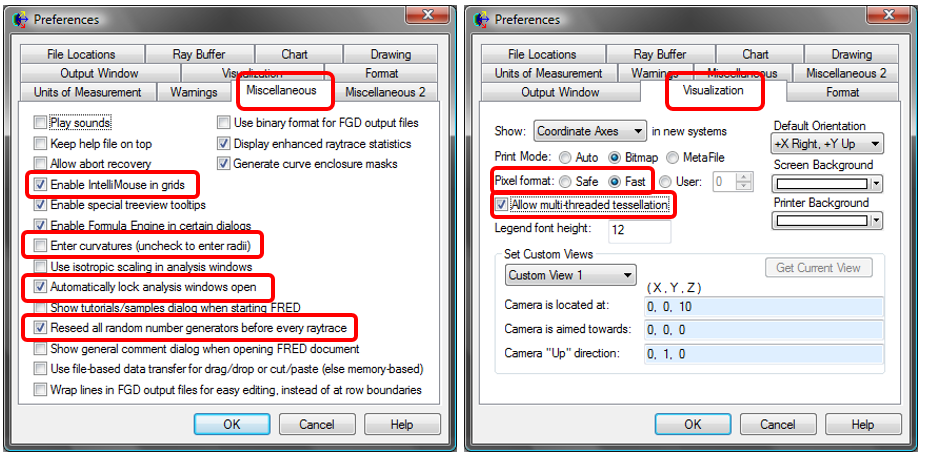
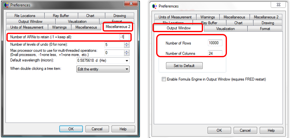
Using the images below as a guide, set each of the preferences as indicated and then hit OK.
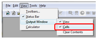
While not explicitly a Preference setting, we also want to make adjustments to the appearance of our Output Window, as indicated below.
When finished making the above changes, close FRED and then restart it. The Preference settings are not saved until FRED is closed.
With the Preferences now set, open a new FRED file by clicking the New Fred Document icon (
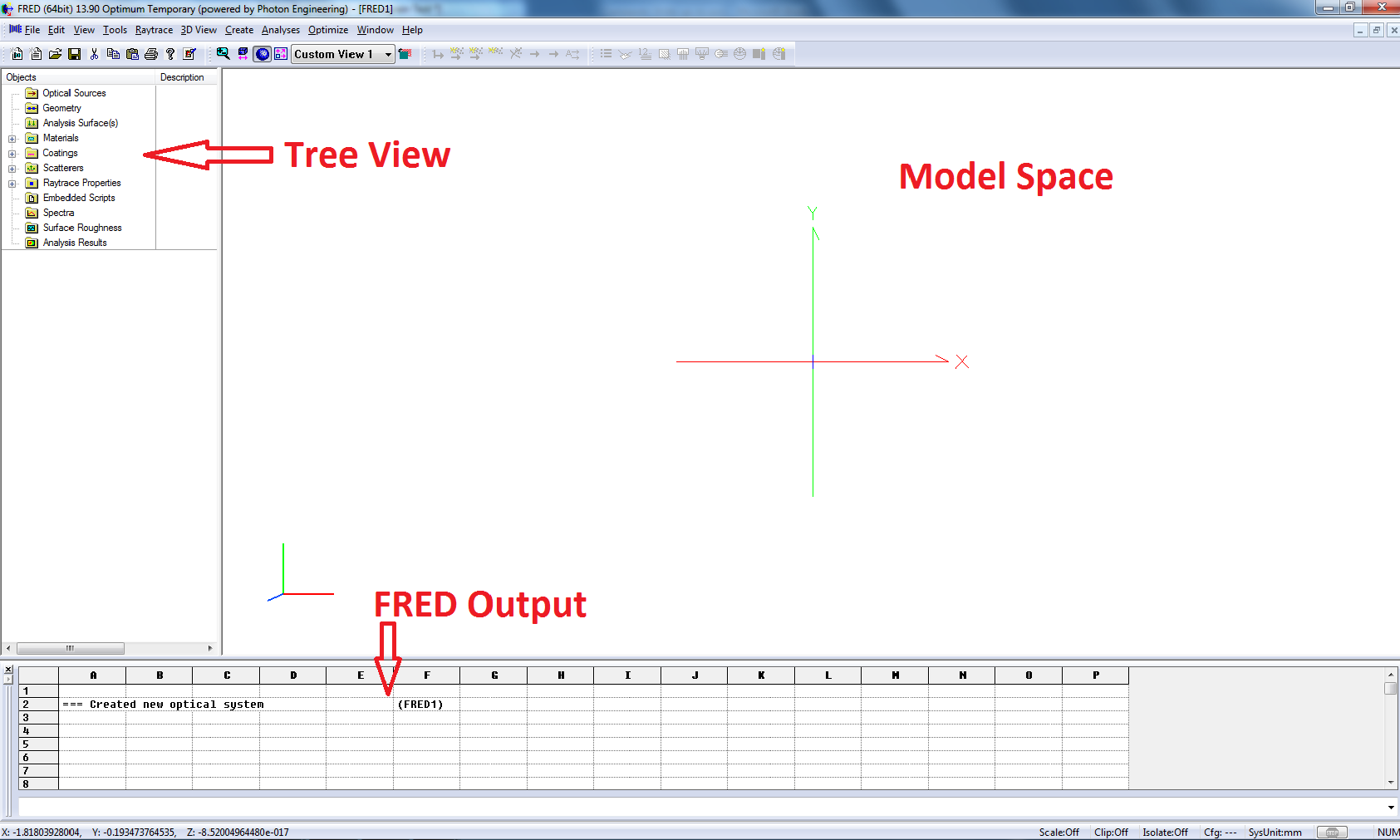
In the newly opened FRED file, notice the object tree that appears on the left side of the screen. This is where all of the lenses, mirrors, sources, coatings, materials, etc. that are in your file will appear to be selected and edited. The right side of the screen will be reserved for displaying the model, while the bottom of the screen is the FRED file output.
Cassegrain telescopes are designed with a parabolic primary mirror having a central aperture and a hyperbolic secondary mirror. This design will not include any field lenses or relay elements. The prescription for the design is provided below in millimeters.
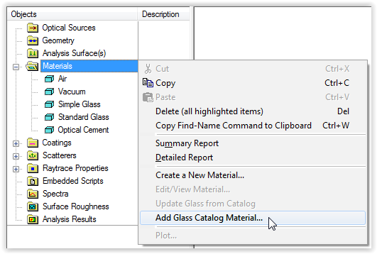
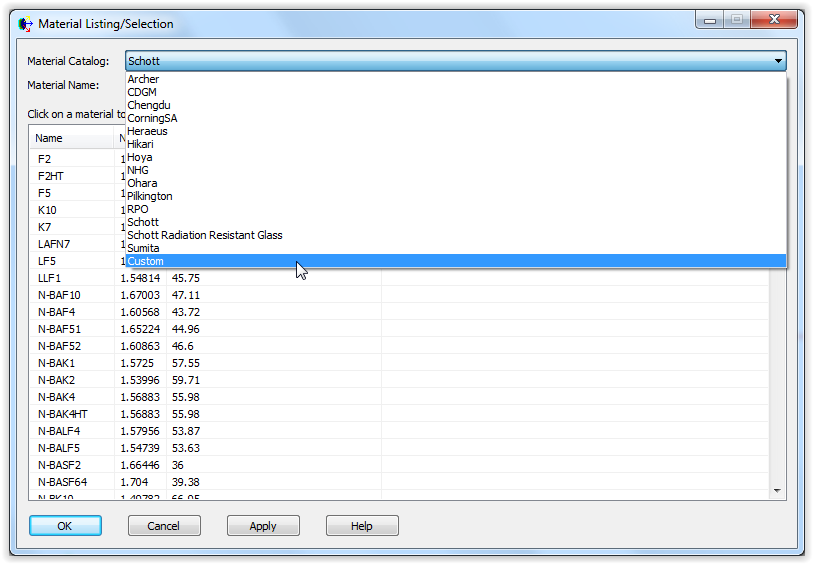
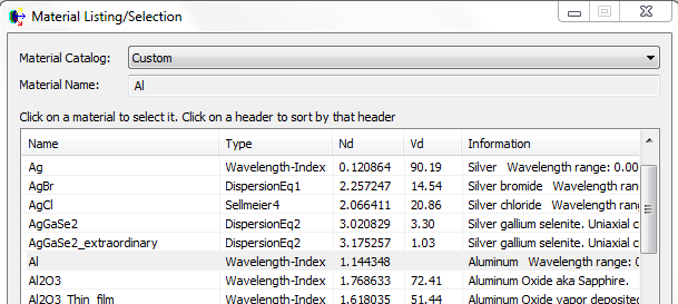
FRED contains many different catalogs of materials and can even but customized to contain user-defined materials. When a FRED document is created, only a small selection of default materials are currently available for use in the document. In your new FRED document, expand the Materials folder to view the handful of materials which are currently available to be used in the document. Additional material definitions can be made available in the Materials folder by right mouse clicking on the Materials folder and selecting “Add Glass Catalog Material”. This will open a dialog that lists all of the available glass catalogs in the drop down list and the corresponding materials for that catalog. For this tutorial, add the "Al" material by choosing the Custom catalog, selecting Al and then hitting the OK button on the dialog.
After adding the Al material you will find that it is now available for use in the Materials folder in the FRED tree view. We will make specific use of this new material in a minute when we create geometry.
A variety of interactions can occur when a ray intersects a surface defined by the geometry, each of which is governed by its own unique surface property. For specular reflection and transmission components, the power leaving the surface in each component is governed by the Coating applied to the surface. There are a variety of ways to define the surface Coating, including reflection and transmission coefficients, digitization of a coating performance curve, entry of a thin film definitions, etc. In this tutorial we will use a simple definition that allows us to specify how much power is directed into the transmitted and reflected components for a given wavelength value.
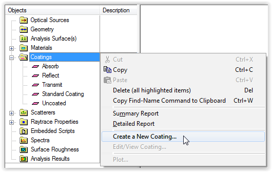
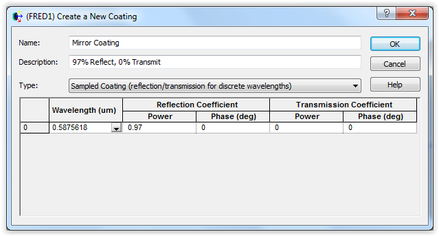
Right mouse click on the Coatings folder of the tree view and select “Create a New Coating” from the context menu. In the resulting dialog, enter the name "Mirror Coating, and select the coating type, "Sampled Coating", from the drop down list item menu. Using the simple Sampled Coating type, we will create a coating that reflects 97% and has zero transmission, as shown below. We will define our coating reflection and transmission values at the default wavelength of .5875618 microns, which is sufficient for this system since it will be modeled with a monochromatic source. In this Sampled Coating definition, if only one wavelength is present in the sampled list then the reflection and transmission values will apply at all wavelengths. If there are multiple wavelengths present in the sampled list, then interpolation is used between sample points to compute the effective reflection and transmission values.
As noted previously with the Materials, after clicking OK to create the coating model you will find that it becomes available for use in the Coatings folder of the tree view. We will apply this coating to the mirror surfaces of our telescope.
Depending on the properties of a given surface interface, power may be distributed among specular reflection, specular transmission, diffraction, or scatter. The properties governing the distribution of power are intrinsic to the definition of the surface itself. However, it may not always be desirable that all of these components be allowed to propagate during the raytrace. In FRED, the Raytrace Property construct is used to control which components should be allowed to propagate during the raytrace. In this sense, the Raytrace Properties are an artificial suppression of components during the raytrace in order to provide the user with a level of control over the raytrace engine. Consider, for example, an interface that has specular reflection 50% and specular transmission 50%. You could apply a Raytrace Property to this interface that only allows the specular transmission component to propagate away from the surface. Note that doing so does not affect the radiometry of the raytrace result, it only indicates that you have no interest in spending CPU time to raytrace the reflected component.
In the FRED Tree View, note that there is a folder called Raytrace Properties and that it contains four default controls. In this tutorial, we will use the default raytrace properties when we construct our system.
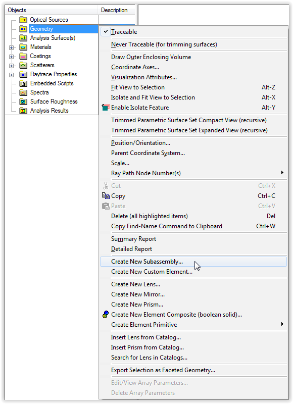
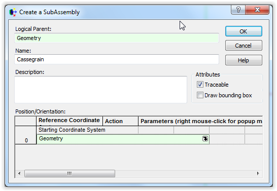
There are constructs in FRED which have no optical properties but which can be useful for organizing other components in the tree view. One such construct is a Subassembly, which simply acts as a storage node for other objects. We start the construction of our geometry by adding a subassembly which will contain all of the components of our telescope. Right mouse click on the Geometry folder of the tree view and choose to "Create New Subassembly" from the context menu. In the resulting dialog, name the subassembly "Cassegrain" and then hit the OK button.
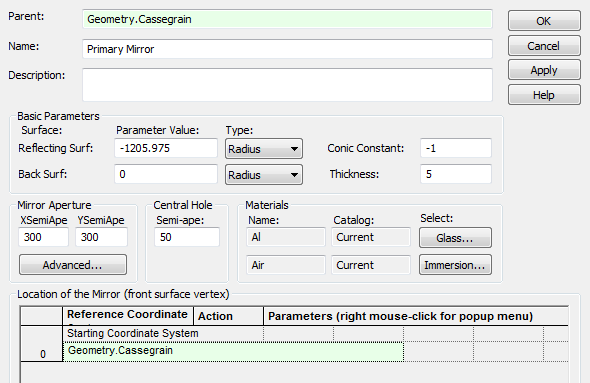
Now that we have added a subassembly node to the Geometry folder, we will add to it the mirror elements and detector for our telescope. First, lets add the primary mirror by right mouse clicking on the Cassegrain subassembly node and selecting "Create New Mirror" from the context menu. In the resulting mirror dialog, note that the construction of the mirror surfaces can be specified in Curvature, Radius, or Focal Length. We will be using the Radius option, which is consistent with the telescope prescription provided earlier. Specify the mirror with the following parameters and then hit OK to add the mirror to the document. Name: Primary Mirror Reflecting Surface Radius: -1205.975 mm Back Surface Radius: 0 mm Conic Constant: -1 Thickness: 5 XSemiApe, YSemiApe: 300 mm Central Hole Semi-ape: 50 mm Glass: Al (added to the document previously)
NOTE: After adding the Primary Mirror element to the system, you may need to re-scale the 3D view to accommodate the new hardware. On the toolbar, right mouse click on the
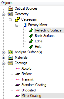
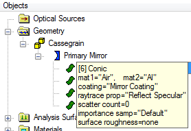
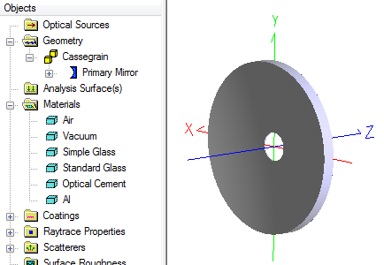
Assigning the Primary Mirror Coating Expand out the Geometry folders until you can see the Reflecting Surface of the Primary Mirror element and then expand out the Coatings folder so that you can see the Mirror Coating that was added previously. Any property can be applied to geometry elements by dragging and dropping the property from its folder onto the target object. If the drop target contains children (ex. the Primary Mirror is a child node of the Cassegrain subassembly node), the property will be applied recursively to all descendants of the target node (ex. all surfaces of the Primary Mirror would inherit the property dropped onto the Subassembly node). In this system, we wish to make the Reflecting Surface of the Primary Mirror have our custom Mirror Coating. This can be done by dragging and dropping the Mirror Coating node onto the Reflecting Surface Node. After the drag and drop is complete, hover your mouse over the green icon of the Reflecting Surface to trigger a tooltip that will display the current properties of that surface. In the 3D view, notice that the vertex of the primary mirror surface is located at the origin of our system.
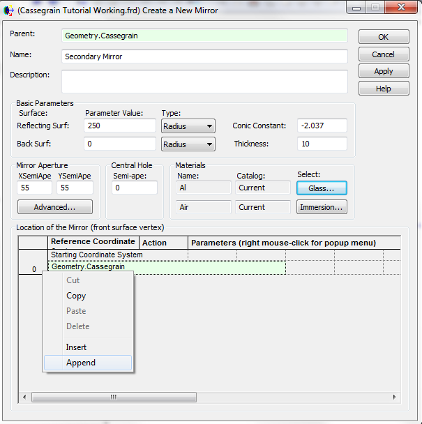
Now that the primary mirror element has been added and has the desired optical properties, we will add the secondary mirror element as defined in our telescope prescription. Right mouse click on the Cassegrain subassembly node and select Create New Mirror from the context menu. In the resulting mirror dialog, enter the following parameters: Name: Secondary Mirror Reflecting Surface Radius: 250 mm Back Surface Radius: 0 mm Conic Constant: -2.037 Thickness: 10 XSemiApe, YSemiApe: 55 mm Glass: Al
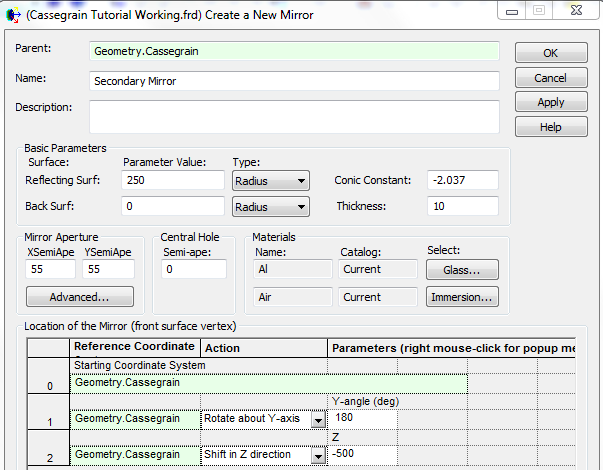
With the mirror optical properties now specified, we additionally need to locate the mirror properly in the model. Our telescope prescription indicates that the vertex-to-vertex distance between the primary and secondary mirror surfaces is -500 mm. We also need to orient the secondary mirror so that the reflecting surface is facing the primary mirror. As shown in the images below, the mirror creation dialog allows for position/orientation operations to be applied to the mirror element when it is created. The mirror begins its life in the coordinate system of the Cassegrain subassembly node. We first append a new operation onto the list, change the operation type to be "Rotate about Y-axis" with a value of 180 degrees. This operation will orient the Secondary Mirror so that the reflective surface is facing the reflective surface of the Primary Mirror. Next, append another operation to the list, change the operation type to be "Shift in Z direction" with a value of -500 millimeters. This sets the vertex-to-vertex mirror separation to the 500 mm specified in our prescription. When finished entering these parameters into the mirror creation dialog, press OK.
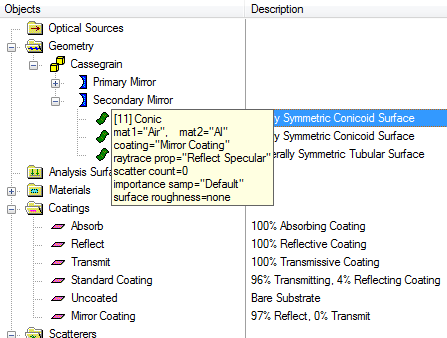
Assigning the Secondary Mirror Coating Using the same drag and drop process described previously for the Primary Mirror reflecting surface, assign the Mirror Coating to the reflecting surface of the Secondary Mirror. After the assignment has been made, hover your mouse over the green icon for the Reflecting Surface of the Secondary Mirror and confirm that the coating assignment has been properly made.
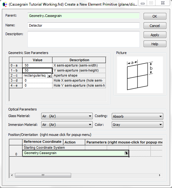
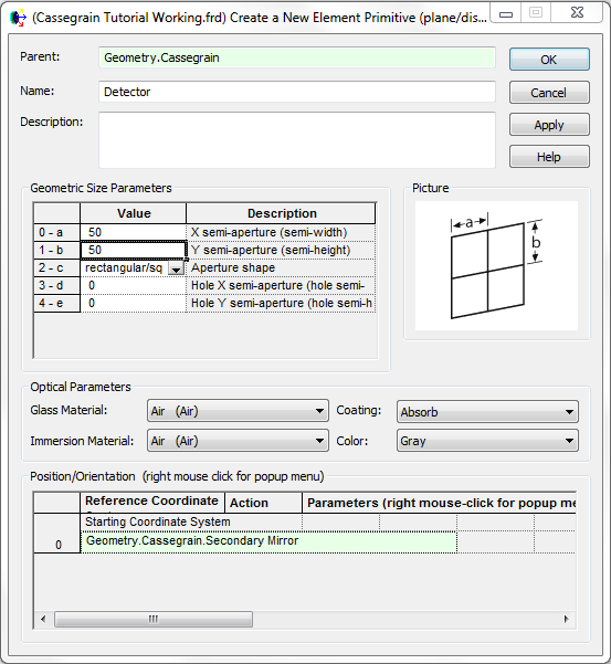
The last piece of hardware that will be added to the model is a representation of the detector. In this case, the detector will be a single plane element with semi-apertures of 50 mm. Right mouse click on the Cassegrain subassembly node and select, "Create Element Primitive", and then "Plane" from the sub-menu. In the resulting Element Primitive Plane dialog, enter the following parameters: Name: Detector X Semi-aperture, Y Semi-aperture: 50
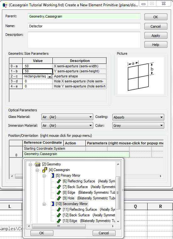
With the detector properties now specified, we need to position the detector in the proper location along the optical axis. According to our prescription, the detector element is located 584.8488682831 mm from the secondary mirror. In the detector dialog, change the starting coordinate system from the Cassegrain subassembly to the Secondary Mirror. Then, right mouse click and append a new operation, changing the type to "Shift in Z direction". The value of the z-shift should be -584.8488682831 (sign flip accounts for the local orientation of the mirror surface in FRED's convention). When finished, press OK on the detector dialog and confirm that it appears in the proper location in the 3D view.
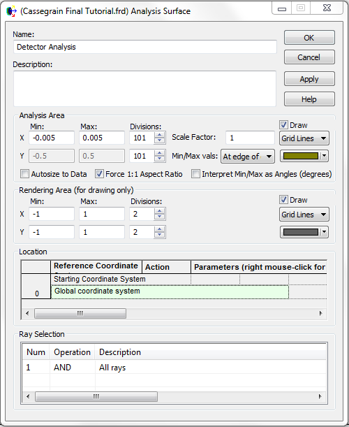
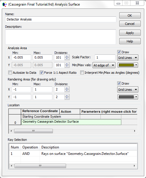
In order to perform analyses, we need to define a grid in space over which an analysis will be computed. The construct which supports this operation in FRED is called an Analysis Surface. Create an analysis surface by right mouse clicking on the Analysis Surface(s) folder and selecting, "New Analysis Surface". In the resulting dialog, enter the following parameters: Name: Detector Analysis Autosize to Data: Unchecked Analysis Area min/max: -0.005, +0.005 Divisions: 101 x 101 After entering the parameters as shown in the dialog below, hit OK to close the dialog.
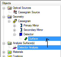
Now that the analysis surface exists on the object tree in the Analysis Surface(s) folder, as shown below, we need to position it at the detector plane. This is easily done by expanding the Analysis Surface(s) folder on the tree so that we can see the Detector Analysis node and expanding the Detector node in the geometry folder so that we can see the detector surface. Once the tree is expanded, we drag and drop the Detector Analysis node onto the Detector.Surface node, as shown below.
This drag and drop assignment of the analysis surface has two effects. First, it positions the analysis surface at the location of the detector plane, which is where we want the analyses to be performed in space. Second, it tells the analysis surface that the rays which should be included in the analysis result are those which ended on the detector surface. You can confirm these two items by opening up the dialog for your analysis surface after the drag and drop assignment and noting the Location and Ray Selection portions of the dialog, as shown below.
At this point, the entire telescope geometry has been constructed and we have added an analysis surface that defines the grid in space over which an analysis will be performed as well as the subset of rays (of all those that exist in the system) which will be used. The last item we need to add to our model is a Source node, which defines the starting set of rays to be traced through the optical system. For this model, we are going to create an on-axis plane wave input to the telescope in the following way:
1. Right mouse click on the Optical Sources folder and select: Create New Source Primitive > Plane Wave (incoherent) 2. In the resulting dialog, set the parameters according to the image shown below.
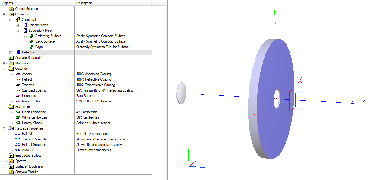
3. Click on the OK button. The 3D view should update to show the newly added source, as shown in the image below.
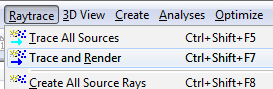
Our system is finally constructed and we are ready to perform some raytracing and analyses. First, perform a raytrace by navigating to Raytrace > Trace and Render. This will create the rays which are defined by the source node, raytrace them through the system and render them in the 3D view.
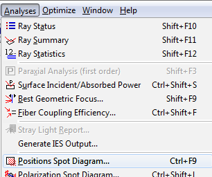
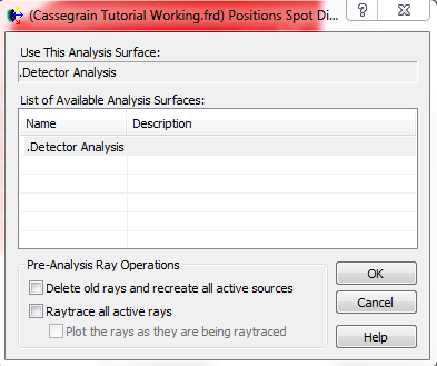
As shown in the 3D view above, the rays have propagated through the system and come to focus at our detector surface. Since we have created and traced rays through the system, we can now call an analysis on the Analysis Surface that we defined earlier. For this demonstration we will calculate the Positions Spot Diagram, which provides statistical information about the geometric ray position data (ex. RMS spot size, average spot size, min/max spot size in x and y, etc.). The Positions Spot Diagram is called by going to Analyses > Positions Spot Diagram. The next dialog that pops up allows you to select which analysis surface you wish to perform the calculation with (we only have one present in this model) and you can simply hit OK. At the end of this process, a chart window will open to display the positions spot diagram graphical result and the statistics of the analysis will be printed to the output window.
This tutorial has demonstrated some fundamentals of FRED's user-interface by working through the construction of a simple Cassegrain telescope model. The concepts introduced apply in the same manner to any other systems constructed in the software.
|
.png)
.png)
.png)
.png)
.png)
.png)
.png)