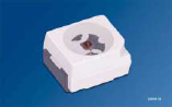
OSRAM TOPLED LS-T676

The goal of this Intermediate Level Tutorial is to move beyond the ideal conditions presented in the Basic Tutorial by 1) modifying the simplistic LED source based upon information from a vendor datasheet, 2) calculating the photometric quantity Illuminance at the lightpipe exit face, 3) introducing FRED's gluing option to apply a prism to the lightpipe exit face which re-directs light exiting the lightpipe, and 4) analyzing ray data using ray path and history features.

Note: The videos included in this tutorial are hosted by YouTube and an internet connection is required to view them.  Controls embedded into the video player will allow you to view the videos in full screen and/or change the video resolution.

A Better Model of LED Characteristics

The goal of this section is to utilize vendor data to more accurately model emission from an LED. We select the TOPLED LS-T676 Super-Red series LED from  OSRAM™ for this exercise. The datasheet for this model can be found on the OSRAM website at this link.  Figure 2-1 shows the spectral power distribution and relative intensity distribution taken from the specification sheet for this LED.

Use a screenshot tool, such as the built-in Windows Snipping Tool, to capture the relative spectral emission curve below and save it to an image file (*.bmp, *.jpg, or *.png file formats).  This image will be used in the build-up of the source model.

Figure 2-1. OSRAM TOPLED LS-T676 LED spectrum (Top) and relative angular power distribution (Bottom).

Begin by right mouse clicking on the existing "Red LED" source node that was generated in the Basic tutorial and selecting the "Traceable" option.  This will deactivate the source node so that its rays are not generated and traced during a raytrace call.

Before we create the new LED source model, we will define the wavelength emission spectrum as a new node in the Spectra folder on the object tree.  Right mouse-click on the Spectra Folder on the object tree and select Create New Spectrum from the context menu. In the resulting dialog, enter the name "OSRAM LS-767" and set the spectra type to be "Sampled" as shown in Figure 2-2. Now right-click in the table area and select the option Digitize Curve.

Figure 2-2. Creating a sampled spectra for the OSRAM LS-T676 TopLED.

The resulting dialog is referred to as the Digitizer, and allows for the extraction of numeric data from an image file.  The general procedure for using the digitizer involves:

1. Load the image into the digitizer interface

2. Calibrate the image by selecting the locations of the origin, x-maximum reference point, and y-maximum reference point

3. Optionally specify whether the axes are logarithmic or polar

4. Select data points on the image for extraction

5. Export the selected data points either (a) back to the FRED dialog from which the digitizer was called, or (b) to a text output file

The movie clip in Figure 2-3 shows the spectra digitization process for the super-red spectrum on the image. Once the process is complete, the digitized data is loaded into the Spectra dialog.

Figure 2-3. Digitizing LED spectra (Video).

We begin by duplicating the existing source to avoid the need to start our source definition from scratch. Open the Optical Sources folder then copy and paste the existing "Red LED" source into the same folder. FRED will automatically name this new source "Red LED 1". Disable the "Red LED" source by right-clicking on its folder definition and selecting the checked "Traceable" entry which removes the check mark and makes the source Untraceable. The "Red LED" source should now appear in the Optical Sources folder with an X over its icon indicating its Untraceable status. Next, double-click on the "Red LED 1" source to open its Detailed Source dialog. Change its name to "OSRAM T676 Red LED" on the Source Tab and hit the Apply button. Leave this Detailed Source dialog box open.

Press OK on the spectrum dialog and see that a new spectrum node called "OSRAM LS-T676" has been added to the Spectrum folder on the object tree.

Now that the spectrum of the source is defined, right mouse click on the Optical Sources folder and choose the option, "Create New Source Primitive > LED (far-field)".  Name this source node, "OSRAM LS-T676 Super Red LED".  The specification sheet of this LED indicates that the typical luminous flux for the S1 brightness group is 0.61 Lumens, which is what we will enter for the Power and Power Units parameters of the Source Primitive specification.  The source will emit a single ray from 100,000 sample positions within the source aperture, which is approximately a 1 mm radius circle based on the specification sheet.  The last parameter of the source specification allows for a custom intensity profile to be applied by using the Digitizer to retrieve data from a polar plot like the one shown on the left side of figure 2-1 (bottom).  For this particular LED, however, the relative intensity distribution is effectively Lambertian.  As the default power apodization of the LED (far-field) type Source Primitive is a Lambertian distribution, there is no need to apply a custom apodization profile to this LED source model.

Finally, we select the "OSRAM LS-T676" spectrum in the Wavelength Attributes portion of the dialog and set the Source Draw Color to be red.  The new source has its starting coordinate system in the Location/Orientation section of the dialog set to be coincident with the original "Red LED" source node.  The final Source Primitive construction dialog is shown below in figure 2-4.  Press the OK button on the dialog to add this new source node to the Optical Sources folder on the object tree.

Figure 2-4. Configured LED (far-field) type Source Primitive dialog.

Illuminance Calculation

In the preceding section, the modified source definition now specifies LED power in photometric units. This allows us to calculate the photometric quantity Illuminance using the same Analysis Surface as was previously used to compute the radiometric quantity Irradiance. The Illuminance calculation is initiated by one of the following methods:

1.From the Main Menu, Analyses>Illuminance

2.Analyses Toolbar button

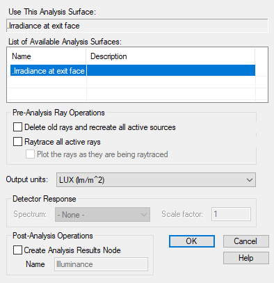
Begin by tracing the source "OSRAM LS-T676 Super Red LED" using Trace All Sources option, thereby avoiding rays being drawn to the screen. Recall that Trace All Sources also uses all available threads (CPUs) resulting in a faster raytrace. Once the raytrace finishes, initiate the Illuminance calculation as indicated above.  Just as with the Irradiance and Intensity calculations made in the Basic Tutorial, a dialog will appear allowing the selection of the analysis surface to be used in the calculation. In the case of an Illuminance calculation, this dialog has a slightly different format as shown in Figure 2-5. In addition to the List of Available Analysis Surfaces and the Pre-Analysis Ray Operations options, the user can select from one of the standard Output Units associated with Illuminance; Lux (lm/m²), phot (lm/cm²), foot-candles (lm/ft²) or lumen/(system unit)². There is also facility for calculation in arbitrary units based upon a Detector Response (see Illuminance Help page for more details on this option). For the purposes of this tutorial, we select the most common Illuminance unit, Lux (lm/m²).

Figure 2-5. Analysis Surface selection dialog for Illuminance calculation.

Figure 2-6 shows the Luminance calculation at the lightpipe exit face again for (Top) 100k source rays and (Bottom) 1M source rays.

Figure 2-6. Luminance calculation at lightpipe exit face for (Top) 100k source rays and (Bottom) 1M source rays

Gluing a Prism to the Lightpipe

This section of the Intermediate Tutorial introduces FRED's unique gluing feature. The most common usage of glue in optical engineering is in construction of doublet and triplet lens. In the context of this tutorial, we demonstrate another common usage of glue; application of a coupling prism to control the direction of light exiting the lightpipe.

Begin this section by adding a prism to the Geometry folder. Create a prism entity by one of the following methods:

1.From the Main Menu, Create>New Prism

2.Keystroke Ctrl+Alt+P

3.Right-click on Geoemtry folder and select Create New Prism

4.Create Toolbar button

The Prism dialog is similar in nature to the Lens dialog used at the beginning of the Basic Tutorial to construct the lightpipe. Both dialogs have Material and Location/Orientation options along with Name & Description fields. Unlike the Lens entity which builds a simple spherical lens by specification of front & back surface radii and center thickness, the Prism is a more complex construct offering sixteen different prism types. The dialog input adapts its parameter set based upon the specific choice of Prism type. For this exercise, select the "General" prism from the Type dropdown list. Specify the Top Angle and Bottom Angle values as 45° & 90°, respectively.  Set the Semi-Aperture of Input Face dimension to span one half of the exit face area, X=10mm and Y=2.5mm. In the Location/Orientation area, set the Reference Coordinate system to that of the exit face and add a z-shift of 0.01mm. Finally, change the Material to PMMA and hit the OK button. The new prism should now appear adjacent to the lightpipe exit face. The movie clip in Figure 2-7 demonstrates this process.

Figure 2-7. Adding a coupling prism to the lightpipe exit face (Video).

One additional step must be performed. Drag-and-drop the Uncoated Coating and Allow All Raytrace Property onto the prism icon in same manner as these assignments were made to the lightpipe in Figure 1-5 of the Basic Tutorial. With these steps complete, we are now ready to glue the prism input face to the lightpipe exit face.

Verify that the prism input face [Prism 1.Surf 1] and lightpipe exit face [Lightpipe.Surface 2] surfaces have the Material assignments PMMA & Air by hovering your mouse cursor over their surface icons in the Geometry folder as was illustrated in Figure 1-4 of the Basic Tutorial. Recall that these surfaced were intentionally given an air gap separation of 0.01mm. FRED's Glue feature is designed to fill this air gap between surfaces with a glue material. For this purpose, a generic "Optical Cement" is included as one of the default entries in the Material Folder of every FRED document. Note, however, that the glue material can be any material in the Material Folder including, in this case, the PMMA from which the lightpipe and prism are made.

Note: Glued surfaces must have a finite separation. As a general rule in FRED, no two surfaces can be coincident. This rule also applies in the case of glue.

Two surfaces are glued together by one of two methods:

•Open the Surface dialog for either surface and navigate to the Glue Tab.

•Right-click on either surface icon in the Tree folder and select the option Glue.

Select the prism input face, Prism 1.Surf 1, and double-click on its icon in the Geometry folder to open the Surface dialog. Navigate to the Glue tab. Specify the lightpipe exit face, Lightpipe.Surface 2, as the surface glued to this surface using the Entity Picker then select the glue material to be Optical Cement. The movie clip in Figure 2-8 below shows this process of gluing the prism and lightpipe.

Figure 2-8. Gluing the prism input face to the lightpipe exit face (Video).

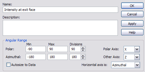
Having succeeded in gluing the prism to the lightpipe, our next step will be to examine the angular distribution of light exiting two of the prism faces: the Output face [Prism 1.Surf 2] and the Bottom face [Prism 1.Surf 3]. The DAE Intensity at exit face used in the Basic Tutorial can be used for this purpose with a few minor changes. We will first re-orient the DAE such that its Polar axis lies along the X direction. In addition, the Azimuthal angle range should be extended to include the entire 4π steradians [-180° to +180°] and the number of Divisions set to Polar=90° and Azimuthal=180°. These setting are shown in Figure 2-9. Finally, the Ray Selection criteria need to be edited to include rays on the prism Output face OR the Bottom face as shown in figure 2-10. 

Figure 2-9. DAE Angular Range settings for Intensity calculation at prism faces.

Figure 2-10. Editing the Ray Selection Criteria to include rays from the Output OR Bottom prism faces (Video).

Our next step will be to make a Luminous Intensity calculation using the newly edited DAE Intensity at exit face after tracing 100k rays from the "OSRAM LS-T676 Super Red LED" source created earlier in this Tutorial. The Luminous Intensity calculation is invoked by one of the following methods:

1.From the Main Menu, Analyses>Luminous Intensity

2.Analyses Toolbar button

Figure 2-11. Luminous Intensity associated with rays exiting the prism Output and Bottom faces.

Figure 2-11 shows a plot of Luminous Intensity in units of Candela using DAE Intensity at exit face. Note the presence of two broader peaks in the azimuthal direction at angles of approximately  -30° and +90°. These features correspond to Snell's Law deviation of the beam exiting the prism Output face [-30°] and the beam exiting the Bottom face in reflection from the Output face [+90°]. This can be verified by eliminating one or the other of the Ray Specifications assigned to the DAE and re-calculating the Luminous Intensity. Note there is no need to re-trace between calculations because this analysis only post-processes the ray data and does not affect the rays during the raytrace. Figures 2-12 and 2-13 show these edited Ray Specifications criterion and the corresponding Luminous Intensity plots which confirm the initial supposition.

Figure 2-12. Luminous Intensity for rays exiting the prism Output face only.

Figure 2-13. Luminous Intensity for rays exiting the prism Bottom face only.

A more curious feature of Figures 2-11,12 & 13 is the presence of regularly spaced peaks at angles along the polar axis. Given the configuration, one might suspect that the width of the prism may be in some way related. With that as our initial proposition, consider now the Luminous Intensity patterns generated when the prism x-width is reduced by half to +/-5mm (Figure 2-14) and then extended again to the full +/- 20 mm width of the lightpipe exit face (Figure 2-15). The ray selection filter has been reset to include rays from coupling prism's Output Face OR Bottom Face.  Also note that the rays must be re-traced prior to performing these analyses, since the coupling prism geometry has been modified and will therefore affect the resulting ray trajectories during the raytrace.

Figure 2-14. Luminous Intensity pattern for prism x-width +/-5mm (half of original width)

Figure 2-15. Luminous Intensity pattern for prism x-width +/-20mm (full lightpipe x-width).

Figures 2-14 & 15 confirm the proposition that the pattern is related to the prism x-width. The bands disappear when the prism spans the full width of the lightpipe and become narrower when the prism width is reduced. We will now examine several diagnostic features in FRED which help visualize the situation which gives rise to these bands. The remainder of this tutorial will introduce features related to ray paths and history.

Our diagnosis process begins with FRED's highly flexible Advanced Raytrace feature. The dialog box for the Advanced Raytrace is opened by one of the following methods:

1.From the Main Menu, Raytrace>Advanced Raytrace

2.Keystroke Ctrl+Shft+A

3.Raytrace Toolbar button

While the dialog associated with this Advanced Raytrace feature shown in Figure 2-16 has numerous options, we will specifically concentrate on the two options Create/use ray history file and Determine raypaths found under Raytrace Options in the top right. Note also that the Draw every option under Output/Drawing Options has been unchecked. Before running the raytrace again, double-click on the source "OSRAM LS-T676 Super Red LED" and set the number of rays to 10k. Reducing the ray count in many cases makes visualization of raypaths more manageable and results in a faster raytrace.

Figure 2-16. Advanced Raytrace dialog configured to determine raypaths, create history file and not draw rays.

When a raytrace is initiated with the Create/use ray history file and Determine raypaths options selected, FRED stores each intersection for each ray in a history file and groups rays into "raypaths" defined by unique sequences of surface intersections. This information is accessed through the Raytrace Paths Summaries dialog found on the Main Menu Tools>Reports>Raytrace Paths. Layout of the Raytrace Paths Summaries dialog is in spreadsheet format as shown in Figure 2-17 where each row represents a unique "path" through the system.

Figure 2-17. Raytrace Paths Summary dialog

Path numbers are listed in the leftmost column and total incoherent power for each path in the second column (filtered vs. total is discussed elsewhere in the Help, but for the purpose of this tutorial they are the same). The rightmost three columns list for each path the Last Entity and First Entity, respectively. These entries tell, in order, where the path started, where the path terminated and the entity intersected prior to the path termination. The remaining columns list information relevant to the path including number of rays (Ray Count), number of intersection (Event Count), etc. Information in this table can be sorted by double-clicking on the header of any given column.

For this particular diagnosis, we are interested in visualizing paths which exit the two faces of the prism, .Prism 1.Surf 2 and .Prism 1.Surf 3. To that end, we first sort the Total Power column forcing the paths containing the greatest power to the top of the list. Next, we sort the Last Entity column to bring together all paths which terminate on the same entity. A cursory examination will show that for .Prism 1.Surf 2, there are over 700 paths and for .Prism 1.Surf 3, over 1800 paths. The vast majority of these paths have only a few rays and therefore contain very little power. For this exercise, our interest lies in the paths which contain the most power. Find the first occurrence of the prism output face [Prism 1.Surf 2] in the "Last Entity" column and highlight that row. Right-click on the highlighted row to reveal a drop-down menu with several options. First select the option "Output Path Details" to print the path intersection list to the Output Window. Right-click again on the highlighted row and select the option "Redraw Ray History" which produces the path visualization by drawing all rays on this specific path in the 3D View. The movie clip in Figure 2-18 shows a demonstration of this process.

Figure 2-18. Examining a raypath. Right-click on row to output path details and redraw ray history to 3D View (Video).

An interesting aspect to the rendered ray path shown in Figure 2-18 is that there appear to be multiple paths within this one path. This apparent inconsistency can be understood by recalling that a ray path is defined as a unique order of intersections. In this case, the Path Details indicate that this path involves nine intersections with .Lightpipe.Edge. Since the .Lightpipe.Edge is formed by the extrusion of a rectangular segmented curve, all four sides are a single entity (Tabulated Cylinder). Therefore, paths from Surface 1 to Surface 2 which contain nine intersections with any of the four sides are indistinguishable.

We leave as an exercise for the user to extend this analysis by examining other paths ending on the prism output face as well as those ending on the prism bottom face. Note that more than one path can be highlighted by holding down either the Ctrl or Shift keys when selecting rows. The same functions available for a single path can be accessed for collections of paths.

This concludes the Intermediate Tutorial section. Save the current configuration to a different file name before proceeding to the Advanced section of this Tutorial.