In this Basic Level Tutorial, users will 1) construct geometry by building a simple slab lightpipe, 2) create a rudimentary LED source, 3) perform basic raytracing, 4) invoke analysis tools such as Ray Summary, Irradiance, Illuminance, and Intensity on a Polar Grid.
Note: The videos included in this tutorial are hosted by YouTube and an internet connection is required to view them. Controls embedded into the video player will allow you to view the videos in full screen and/or change the video resolution.
Building Lightpipe Geometry Begin the Tutorial by opening a blank FRED document (File>New>Fred Type, keystroke Ctrl+N or Toolbar button
Figure 1-1. New FRED document.
This tutorial begins by creating a simple rectangular lightpipe from the FRED Lens entity. The Lens entity in FRED is a special construct from which all the pertinent parameters of a simple lens can be entered in a single dialog. Create a new Lens by one of four methods:
1.From the Main Menu, Create>New Lens 2.Keystroke Ctrl+Alt+L 3.Create Toolbar button 4.Right-click on either a Subassembly or the Geometry folder and select option Create New Lens
In this case, the Lens surfaces are planar (radius=0) and the thickness determines the lightpipe length. The X & Y semi-ape under Lens Aperture Specification determines the cross sectional dimensions of the lightpipe. Since the default cross section of a Lens is elliptical (circular), the Advanced Settings button the under Lens Aperture Specification must be selected to access the setting which produces a rectangular cross section. The lightpipe used in this tutorial will have length 100mm with width(X) 40mm and height(Y) 5mm. Our lightpipe material will be PMMA found in FRED's Custom material catalog. A short clip shown in Figure 1-2 demonstrates the construction of the lightpipe to these specifications.
Figure 1-2. Creating a simple lightpipe from the Lens dialog (Video).
After selecting 3D View > View All, we now have the lightpipe as shown in Figure 1-3. Note that if the View All option in the 3D View menu is grayed out, you must click in the 3D view to activate that pane of the application and then revisit the 3D view menu. It can be seen that the PMMA material that was selected in the Lens dialog has been added to the Materials folder in the Tree.
Figure 1-3. PMMA lightpipe from Lens entity.
Note: To assure newly added geometry is entirely visible, it may be necessary to use the View All feature. Keystroke F10 or the Toolbar button
Let us now examine the properties of the lightpipe surfaces. Hover the mouse cursor over the surface icon
Figure 1-4. Check surface properties by hovering over its Tree icon (Video).
Realistic properties of these surfaces should allow for reflection, transmission and total internal reflection characteristic of the bare substrate material. Therefore, each of the surfaces must be assigned the Uncoated coating and an Allow All Raytrace Property. These changes are made by dragging-and-dropping the Uncoated coating and Allow All Raytrace Property onto the lightpipe Lens entity icon
Figure 1-5. Drag-and-drop Coating and Raytrace Properties (Video).
Simple LED Source
The most simplistic model of an LED consists of a Lambertian source with the appropriate spatial dimensions, wavelength and power. Such a source can be quickly created in FRED by using the Lambertian Plane type of Source Primitive. A source of this type can be created using one of the following methods:
1.From the Main Menu, Create > Source Primitive > Lambertian Plane 2.Right-click on Optical Sources folder in Tree and select Create New Source Primitive > Lambertian Plane 3.Create Toolbar button icon:
Figure 1-6 shows the dialog for the Lambertian Plane type of Source Primitive. There are 10 parameters that describe the source power, spatial ray distribution and angular ray distribution, as well as the emission wavelength(s) and location/orientation of the source in the model. In this example, the source will emit 100K rays monochromatically at 0.625 microns from a Lambertian plane with a 0.2 mm rectangular aperture and the ray emission will subtend a cone angle of +/- 80 degrees. The source emits 0.045 Watts of power and is located -0.1 mm from the entrance face of the lightpipe. The video in figure 1-7 demonstrates how to set the location/orientation of the source node.
Figure 1-6. Source Tab for Detailed Source.
Figure 1-7. Reference LED position relative to lightpipe entrance face (Video).
Basic Raytrace
We are now in position to trace the source rays through the lightpipe. While there are numerous options for raytracing in FRED, we restrict ourselves at this stage to a basic raytrace initiated by one of three methods:
1.From the Main menu, Raytrace>Trace and Render or Raytrace>Trace All Sources 2.Keystroke Ctrl+Shft+F7 or Ctrl+Shft+F5 3.Raytrace Toolbar button
The Trace and Render option creates rays according to the source definition and performs the trace drawing each ray's trajectory in the 3D View. The Trace All Sources option creates rays according to the source definition and performs the trace without drawing the ray trajectories. The difference between drawing and not drawing the ray trajectories carries two important consequences:
Since illumination simulations often require tracing rather large numbers of rays, the Trace All Sources option is preferred in virtually all situations. Common practice is to first trace a modest number of rays with the The Trace and Render option to confirm the model is set up correctly then increasing the number of rays and using the Trace All Sources option.
This simple geometry and source serve as a meaningful example of the difference in raytrace time between these two options. Using a dual core laptop with 4 threads, tracing 100,000 rays with the Trace and Render option took 12 seconds using a single thread as indicated in Figure 1-8. With the Trace All Sources option, the same number of rays traced in 1.85 seconds using four threads as indicated in Figure 1-9.
Figure 1-8. Raytrace Summary after Trace and Render.
Figure 1-9. Raytrace Summary after Trace All Sources.
Note that the entry "Num rays halted due to exceeding number of consecutive intersections on the same surface (info:3)" appears in both Figures 1-8 and 1-9. This message will be discussed in the following section in context of our analyses of the system.
Analyses
The Ray Summary is always a useful top-level tool for assessing results. This feature is invoked by one of three methods:
1.From the Main Menu, Analyses>Ray Summary 2.Keystroke Shft+F11 3.Analysis Toolbar button
After pressing OK on the dialog that opens, the Ray Summary prints to the Output window a complete listing of number of rays and total incoherent power on each surface along with the surface name. After raytracing the lightpipe, Ray Summary produces an output shown in Figure 1-10. [Your result may differ slightly as the source is a random source whose positions and directions have been chosen by FRED's random number generator and are different for each raytrace instance.]
Figure 1-10. Ray Summary after raytrace of lightpipe.
Aside: Ancestry and the Raytrace Properties
Two points should be evident from the output shown in Figure 1-10 in connection with the raytrace from the previous section:
•If the Trace and Render option is used, one will observe that no rays exit the Lightpipe.Edge surface, yet the Ray Summary shows power of ~0.01 on that surface (>20% of total LED power). The presence of this entry can be related directly to the "exceeding number of consecutive intersections" message highlighted in the previous section.
•The total power tabulated in Figure 1-13 (0.044976, last row, second column) is slightly less than the total power assigned to the LED source (0.045).
An understanding of these two points is found in the Allow All Raytrace Property assigned to each surface. The dialog for this property is shown in Figure 1-11. The Intersection Count Cutoff settings address the first point. The entry, Consecutive, restricts the number of consecutive intersections with the same surface. While the default value of 10 is reasonable for many applications, modeling lightguides often requires the Consecutive entry to be increased. While some trial-and-error is inevitable, the user should increase this value in an incremental fashion until the "exceeding number of consecutive intersections" warning no longer appears in the Raytrace Summary.
Figure 1-11. Allow All Raytrace Properties dialog (default).
For this example, the warning is eliminated when Consecutive entry be increased to 20. After re-tracing the rays, the Ray Summary shown in Figure 1-12 shows rays only on the Surface 1 and Surface 2, the entrance and exit faces of the lightpipe, respectively.
Figure 1-12. Ray Summary after Consecutive setting on Allow All Raytrace Property increased to 20.
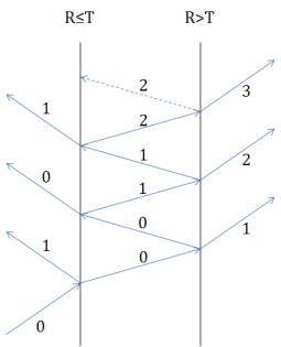
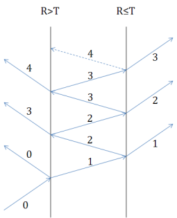
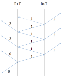
With regard to the second point above, note that the Total Incoherent Power is still about 0.15% less than the assigned source power of 0.045. This slight discrepancy results from the Ancestry Level Cutoff option on the Raytrace Property. The term ancestry incorporates the concept of generations commonly associated with parent, child, grandchild, etc. These generations may also be denoted numerically as 0,1,2,3..... Figure 1-13 illustrates generational splitting in four distinct cases when a single ray is incident upon successive surfaces. The Ancestry Level Cutoff option halts creation of rays beyond the given generation. The default specular ancestry for all Raytrace Property controls is set to 2 meaning that up to two specular generations are allowed. The termination of generations higher than 2 is therefore the reason for the 0.15% power discrepancy. Since these generations are not created, the power associated with them is permanently lost in the power accounting process.
(a)
(c) Figure 1-13. Ancestry splitting of incident parent (0): a) R≤T both surfaces, b) R≤T, R>T, c) R>T, R≤T, d) R>T both surfaces.
Irradiance & Intensity
Commonly used metrics for evaluating optical system performance are Irradiance and Radiant Intensity. Their photometric equivalents are Illuminance and Luminous Intensity, respectively. Irradiance and Illuminance are measured in units of flux per unit area while Radiant Intensity and Luminous Intensity are measured in units of flux per solid angle. These are among a larger group of what are generally referred to as "Energy" calculations in FRED. Table 1-1 below lists these basic radiometric and photometric quantities along with their common units. Irradiance and Illuminance calculations require an Analysis Surface (AS). Radiant Intensity and Luminous Intensity calculations require a Directional Analysis Entity (DAE).
Table 1-1. Radiometric/Photometric Quantities and Units
* - Irradiance units will be expressed with area units given by the current system units in the FRED document.
The Analysis Surface
Figure 1-14. Analysis Surface in FRED's 3D View.
The Analysis Surface is a planar area used to make an Irradiance calculation. Its representation in the 3D View is shown in Figure 1-14 and dialog box in Figure 1-15. The Analysis Area option sets the local X & Y extents which define a rectangular area, the number of pixels (divisions) in each direction, a scale factor applied equally to the X & Y extents, as well as autosize and 1:1 aspect ratio settings. The user can also choose whether to draw the Analysis Surface grid in FRED's 3D View and to interpret X & Y extents as being at the edge or center of the outer pixels.
The Location option for an Analysis Surface determines the Reference coordinate system in which the calculation is to be performed. While the default is the Global coordinate system, generally the coordinate should be that of a specified surface. The Ray Selection option determines which rays are to be used in the calculation. While the default is All rays, only those rays currently on the surface of interest should be selected. Both the Location and Ray Selection can be set manually or set simultaneously by drag-and-drop of the Analysis Surface onto the surface of interest. For more detailed explanation of Analysis Surface options, navigate to its Help page using this link Analysis Surfaces.
An Analysis Surface is created using one of the following methods:
1.From the Main Menu, Create>Analysis Surface 2.Keystroke Ctrl+Alt+N 3.Right-click on Analysis Surface(s) folder and select option New Analysis Surface 4.Create Toolbar button
Figure 1-15. Default Analysis Surface dialog.
Note: Analysis Surfaces and Directional Analysis Entities are not surfaces in the strict sense of an absorbing/reflecting/transmitting/scattering/diffracting surface in your optical model. Rays are not absorbed by an Analysis Surface or a Directional Analysis Entity. These constructs serve only to demarcate and subdivide an area or range of directions over which calculations occur. These constructs only post-process ray data after the raytrace has occurred, but do not interact with the rays in any way during the raytrace itself.
Directional Analysis Entity
Figure 1-16. Directional Analysis Entity in FRED's 3D View.
A Directional Analysis Entity measures Intensity over the full 4π steradians in equal angle increments. Its graphic representation in the 3D View is shown in Figure 1-16 and its dialog box in Figure 1-17. The Directional Analysis Entity is represented graphically in the 3D View as a sphere whose polar and azimuthal divisions are analogous to longitudinal and latitudinal lines on a world globe. The terms "polar" and "azimuthal" therefore must be distinguished from their conventional meanings in a spherical coordinate system. The Polar axis runs from the "north" to "south" poles of the globe and is chosen by the user to lie along one of the three local coordinate system axes. The "azimuthal" angle is measured from the user-selected Other Axis coordinate axis direction.
As with the Analysis Surface, the Location option for the Directional Analysis Entity determines the Reference coordinate system in which the calculation is to be performed. While the default is the Global coordinate system, generally the coordinate should be that of a specified surface. The Ray Selection option determines which rays are to be used in the calculation. While the default is All rays, only those rays currently on the surface of interest should be selected. Both the Location and Ray Selection can be set manually or set simultaneously by drag-and-drop of the Directional Analysis Entity onto the surface of interest. For more detailed explanation of Directional Analysis Entity options, navigate to its Help page using this link Direction Analysis Entity (DAE).
A Directional Analysis Entity is created using one of the following methods:
1.From the Main Menu, Create>Directional Analysis Entity 2.Keystroke Ctrl+Alt+Y 3.Right-click on Analysis Surface(s) folder and select option New Directional Analysis Entity 4.Create Toolbar button
Figure 1-17. Default Direction Analysis Entity dialog.
Having been introduced to the these basic tools for analyzing our results, we shall now make the lightpipe model ready for an Irradiance and an Intensity on a Polar Grid calculation at the exit face. The initial step involves adding then "attaching" both an Analysis Surface and a Directional Analysis Entity to the lightpipe exit face "Geometry.Lightpipe.Surface 2". The movie in Figure 1-18 shows a clip in which an Analysis Surface is attached to the exit face via the drag-and-drop method. The movie in Figure 1-19 shows a clip in which a Directional Analysis Entity is attached in the same manner. The default size and pixel settings are used for this initial step, but we will return to the dialogs later to update those settings.
Figure 1-18. Creating and attaching an Analysis Surface to lightpipe exit face (Video).
Figure 1-19. Creating and attaching a Directional Analysis Entity to lightpipe exit face (Video).
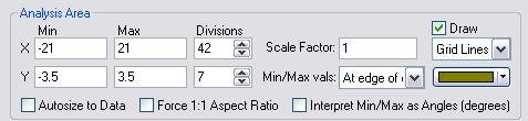
To more clearly display the Irradiance calculation, we choose to make some changes to the Analysis Surface default Analysis Area settings as shown in Figure 1-20. The intent will be to create 1mm2 pixels with a padding of one millimeter in both dimensions. Forcing the outer pixels to zero produces a more pleasing contrast between minimum and maximum. To that end, the Autosize to Data and Force 1:1 Aspect Ratio options must be disabled[unchecked]. Next, the Min & Max values in X and Y are set to [-21,+21] and [-3.5, +3.5], respectively. Note that the Min/Max vals option default setting indicates that these dimensions are measured At edge of outer pixel. Based upon theses X & Y dimensions, the number of Divisions must be set to 42x7 to achieve 1mm2 pixels.
Figure 1-20. Analysis Surface parameter settings.
With the Analysis Surface configured as above, we now run an Irradiance calculation. An Irradiance calculation is invoked using one of the following methods:
1.From the Main Menu, Analyses>Irradiance Spread Function 2.Keystroke Ctrl+F10 3.Analysis Toolbar button
The call for an Irradiance Spread Function pops a dialog as shown in Figure 1-21. This dialog allows the user to select among the available Analysis Surfaces which is to be used for the calculation. Here we have only one to choose from; Irradiance at exit face. However, in general, any number of Analysis Surfaces can be defined and all will be presented in this list when the Irradiance Spread Function is requested. The user must select the specific Analysis Surface to be used for the current calculation. Note also the Pre-Analysis Ray Operations options. If a raytrace has been executed prior to the Irradiance Spread Function request, then these options are unchecked. The user simply selects the OK button to proceed. On the other hand, if the Irradiance Spread Function is requested before any raytrace, these options allow for the raytrace to be executed from this dialog before the calculation proceeds.
Figure 1-21. Analysis Surface selection dialog.
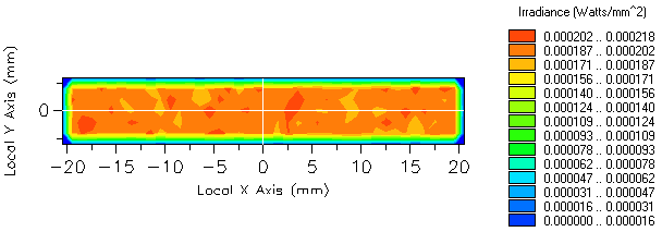
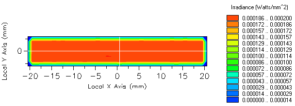
The resulting irradiance at the lightpipe exit face calculated with a) 100k and b) 1000k rays is show in Figure 1-22 (the ray counts can be increased by editing the source node and modifying the number of starting ray positions). These results offer an opportunity to highlight the statistical aspect of "Energy" calculations which is particularly applicable to illumination. Since the source is traced as a set of randomly-generated ray positions and directions, "Energy" calculation results are governed by Poisson statistics which states that the signal-to-noise ratio associated with each pixel is proportional to √N where N is the number of rays per pixel. Examination of the plot levels reveals the predicted 3x decrease in peak-to-valley variation across the central portion of the irradiance patterns between a) and b).
(a)
(b) Figure 1-22. Irradiance at lightpipe exit face with a) 100k rays and b) 1000k rays.
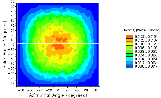
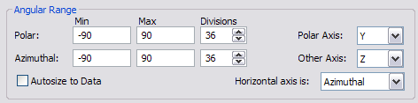
Next, we calculate the Intensity at the exit face using the Intensity on a Polar Grid analysis feature. Since rays can only leave the exit face in the +z direction, the Directional Analysis Entity should be edited in order to restrict the calculation to that hemisphere. For the default polar (Y) and azimuthal (Z) axes in the local coordinate system, the azimuthal angle should range from -90 to +90 deg as shown in Figure 1-23.
Figure 1-23. Directional Analysis Entity settings for Intensity calculation at lightpipe exit face.
An Intensity on a Polar Grid calculation is invoked using one of the following methods:
1.From the Main Menu, Analyses>Intensity on a Polar Grid 2.Analysis Toolbar button
The call for an Intensity Spread Function pops a dialog as shown in Figure 1-24. This dialog allows the user to select among the available Directional Analysis Entities which is to be used for the calculation. Here we have only one to choose from; Intensity at exit face. However, in general, any number of Directional Analysis Entities can be defined and all will be presented in this list when the Intensity Spread Function is requested. The user must select the specific Directional Analysis Entity to be used for the current calculation. Note also the Pre-Analysis Ray Operations options. If a raytrace has been executed prior to the Intensity Spread Function request, then these options are unchecked. The user simply selects the OK button to proceed. On the other hand, if the Intensity Spread Function is requested before any raytrace, these options allow for the raytrace to be executed from this dialog before the calculation proceeds.
Figure 1-24. Directional Analysis Entity selection dialog.
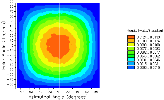
Figure 1-25 shows the Intensity calculation for the same two cases as above; 100k and 1000k rays. Again note the increase in SNR resulting from increasing the ray count by 10x.
a)
b) Figure 1-25. Intensity on a Polar Grid calculation at lightpipe exit face for a) 100k rays and b) 1000k rays.
This concludes the Basic Tutorial. Save the system as a FRED document before proceeding to the Intermediate Tutorial.
|
.png)
.png)
.png)
.png)
.png)
.png)
.png)
.png)
.png)
.png)
.png)
.png)
.png)
.png)
.png)