This Help article draws heavily from the "Intro To FRED Distributed Computing" RTF document, written and maintained by the FRED development team, which can be found in your FRED installation directory under the <install dir>\Resources\Samples\DistributedComputing folder.
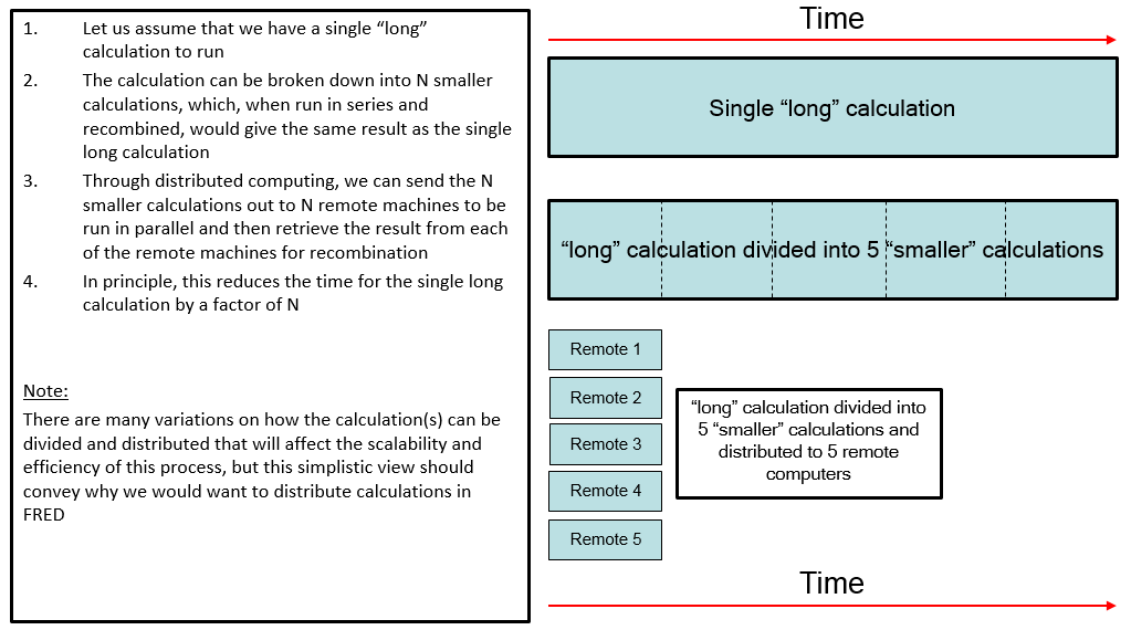
The architecture of FRED distributed computing is implemented in a very flexible way so that any calculation FRED can perform as a stand-alone instance can also be performed as a distributed computation. Any license authorized for use of FRED Optimum is allowed to use the distributed computing capability. The graphic below illustrates the concept of distributed computing, where the time spent for a given calculation running on a single computer can be dramatically reduced by splitting the calculation among any number of computers running in parallel. Many analyses performed in FRED require millions (or even billions) of rays to generate sufficient statistics in the calculation or require an analysis to be repeated for many configurations (or a combination of these two scenarios). In either case, the processing time can be significant and distributed computing offers a way to parallelize your analyses in a manner that is only limited by the availability of Windows computers on your network.
How Distributed Computing Works in FRED What FRED Distributed Computing Is What FRED Distributed Computing Is NOT How Master-Remote Communication Works
What FRED Distributed Computing Is The architecture of FRED's distributed computing capability is implemented in a very flexible way so that any calculation which can be run on a stand-alone FRED instance can also be run as a distributed calculation across a Windows network. Only FRED Optimum licenses will allow access to the distributed computing functionality and only one license is required (the computers being distributed to do not require individual licenses).
Distributed computing is implemented through FRED's BASIC scripting language by running a script on a "master node" that handles distribution of the calculation over the Windows network to one or more "remote instances". In a typical setup, the remote instances are instructed by the master node to execute their own analysis scripts, generate results files, and return the results files to the master node for recombination into a final, composite analysis result.
Ignoring the specifics of installation and establishing communication between master node and remote instances, the core of a master node script controlling the distributed calculation may be as simple as:
What FRED Distributed Computing Is NOT FRED's implementation of distributed computing is not a low-level operation that automatically and transparently distributes primitive FRED calculations (such as a ray trace) to multiple remote nodes. In this sense, it is not analogous to multi-threading. Rather, the user is required to write a specialized script being run on the master node that provides explicit instructions for the remote instances.
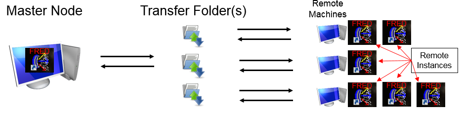
Ignoring, for a moment, how the communication between the master node and the remote instances actually works, there are three network components that are required to run a distributed computation. These items are described below, with the graphic indicating the flow of information across the network.
Master Node A master node is a running instance of FRED Optimum and the user initiates a distributed computing calculation by executing a specific FRED script that has been written to manage the distributed calculation. For this purpose, the scripting language has been extended to include a relatively small number of specialized commands referred to as IPC (Inter-Process Communication) commands. Full documentation of these IPC scripting commands can be found in the Scripting Reference Manual as well as in the IntroToFREDDistributedComputing.rtf document found in the <install dir>\Resources\Samples\DistributedComputing folder. The script being run to manage the distributed calculation, which we will refer to as the "master script", will typically take the following sequence of actions:
Transfer Folder(s) The transfer folder(s) are locations on the network, accessible by both the master node and each individual remote instance, used as intermediate locations for passing files between master and remote. When a file is pushed from the master node to a remote, the process is actually completed in two steps; (1) master node pushes file to the transfer folder associated with the destination remote, and (2) destination remote pulls the file from the transfer directory to its local working directory. The operations is similar when the master requests a file to be pulled from the remotes; (1) remote pushes a file to its associated transfer folder, and (2) the master node pulls the file from the transfer directory to its working directory. In reality, there is no requirement that each remote have its own unique transfer folder. A single transfer folder can be used for multiple remotes as long as it is accessible to all of them. The file push process is illustrated in the graphic below.
Remote Instance(s) Remote instances, when successfully launched by a master script, listen for instructions being sent to them by the master node in the form of IPC script commands. IPC scripting commands direct the remote instance to perform specialized tasks that ultimately result in generation of output files that can be returned to the master node. Such instructions include IPCLoadModel (instructs the remote instance to load a specific FRED file), IPCExecEmbeddedScript (instructs the remote instance to execute a specific embedded script in the currently loaded model), and IPCPullFile (copy a specific file from the remote machine across the network to the master node). Remote instances do not require access to a FRED hardware key, license services, or drivers, though FRED does need to be installed on each of the remote machines. The only software license required is a FRED Optimum license accessible by the master node.
How Master-Remote Communication Works Communication between the master node and remote instances works through the use of Windows "named pipes", which are simply conduits for communication between sever (the process that created the pipe) and client (the process that connects to the pipe) and subject to Windows security checks and authorization. When a remote instance of FRED is started, it creates a pipe, the master node connects to the pipe, and the IPC commands flow through the pipe from master to remote.
According to the available documentation, named pipes may use UDP ports 137-139 and/or TCP 445. Network administrators are responsible for ensuring that the Windows firewall and other network protection settings allow communication through named pipes over these ports.
There are two methods of establishing the initial connection between master node and remote instances; the appropriateness of a given method depends on the specific security settings and software installed on your Windows network. The installation and requirements for each method is described in another section of this document. Please contact your network administrator with any questions regarding your network policies.
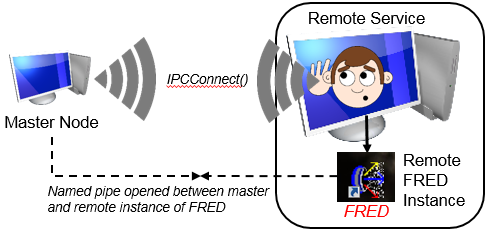
Method 1: FRED Remote Service The FRED Remote Service is an optional service that runs on the remote machines to facilitate communication between master node and remote machine. When started, the FRED Remote Service creates its own named pipe and listens on it for connection requests coming from a master node. A master script, managing the distributed calculation, will send out an IPCConnect() request to a remote machine using the named pipe created by the FRED Remote Service. When an IPCConnect() request is received by the FRED Remote Service, it asks Windows to authenticate the user account that initiated the request and, if the account is validated by Windows, it creates a temporary local working directory on the remote machine before launching a new remote FRED instance. Once the remote FRED instance is launched by the FRED Remote Service, a new named pipe is created by the remote FRED instance, the information about the named pipe is passed back to the master node via the FRED Remote Service, and the master node can then communicate directly to the remote FRED instance on the dedicated named pipe between them. Having established communication directly between the remote FRED instance and the master node, the FRED Remote Service has performed its function and returns to listening for IPCConnect() requests over its own named pipe. In this way, the FRED Remote Service is capable of starting as many remote FRED instances on its own machine as requested by a master node, as long as the local computer resources can support them. Communication between a master node, FRED Remote Service and remote FRED instance is illustrated in the graphic below.
Method 2: MPICH MPI (Message Passing Interface) is a third party standard commonly used to facilitate classical distributed computing. While FRED is not a native MPI application and does not use MPI for communication between the master node and remote instances, it can use MPI utilities to launch FRED instances on the remote machines as a substitute for the functionality provided by the FRED Remote Service. In some network environments the use of the FRED Remote Service may be prohibited due to account restrictions. In such cases, the MPI method may be required.
MPI is an open standard (to some degree) and different "flavors" of MPI are available from various sources, some of which can be downloaded for free and used with restriction, while others may involve a fee. Some MPI flavors we are aware of are MPICH, Open MPI, Intel MPI, Microsoft MPI, etc. This list is not meant to be exhaustive. Many flavors of MPI may work with FRED, but certain aspects of installation and usage may be unique to each.
The MPI utilities are used solely for their ability to launch applications on remote machines in response to the proper request from a master machine. MPI plays no further role once the remote instances have been launched.
The MPI utilities perform several tasks when launching a Remote:
Some advantages of using the MPI launch method are:
Some disadvantages of using the MPI launch method are:
The installation procedure for distributed computing is different for the FRED Remote Service and MPICH methods. Only one method is required and the installation for each method is described separately below. Please keep in mind that Windows networks come in a wide variety of configurations and Photon Engineering cannot anticipate every installation scenario. Consequently, your installation process may be different than that shown here and you may need to involve your local IT administrator in order to identify any specific issues during installation.
Installation Procedure for using the FRED Remote Service
Installation Procedure for using MPICH MPI (Message Passing Interface) is a third party standard commonly used to facilitate distributed computing. While FRED is not a native MPI application and does not use MPI for communication between the master and remotes, it can use MPI utilities to launch remote FRED instances as a substitute for the functionality of the FRED Remote Service. See "How Master-Remote Communication Works" above for more information.
MPI is an open standard and different "flavors" of MPI are available from various sources, some of which can be downloaded for free and used without restriction, while others may involve a fee. Some MPI flavors we are aware of are MPICH, Open MPI, Intel MPI, Microsoft MPI, etc. This list is not meant to be exhaustive. Many flavors of MPI may work with FRED, but certain aspects of installation and usage may be unique to each.
FRED Distributed Computing has been successfully tested with MPICH, and the information provided below provides a summary description of how MPICH may be installed for use with FRED Distributed Computing. We first describe how to install FRED on the master and remote machines, followed by a description of how to install MPICH for use with FRED.
Installation of FRED on the Master Machine Follow the normal FRED installation procedure on the master machine. The "Remote Service" installation option does NOT need to be toggled.
Installation of FRED on the Remote Machine(s) Follow the normal FRED installation procedure on each remote machine. The "Hardware Key" and "Remote Service" installation options do NOT need to be toggled.
MPICH Installation on the Master and Remote Machines Photon Engineering does not distribute or install MPICH as part of the FRED installation. We recommend the user examine the documentation that can be found on the www.mpich.org website for complete information, since the user is ultimately responsible for download and installation. A summary description of the relevant installation details is given below.
When a distributed calculation is run in FRED, there is no requirement that the remote computers performing the calculation have the same hardware and, therefore, the same computing power. In other words, FRED's distributed computing capability can be run on an inhomogeneous Windows network. If, in the simplest case, a raytrace of the same exact FRED model is performed simultaneously by an inhomogeneous set of remote computers, you would expect that the more powerful computers will finish the raytrace faster than the less powerful computers. Since the master computer will be waiting to pull the calculation result from all of the remote instances, the distributed calculation time is limited by the slowest remote instance. This type of configuration is inefficient because the powerful computers are sitting idle while they wait for the slowest computers to finish.
Load balancing is the idea that we can distribute the total workload of the calculation unevenly across all of the remote instances, accounting for their relative performance. For example, suppose that a calculation is distributed to two remote instances in which Remote1 is twice as fast as Remote2. For maximum efficiency, we would want to "load balance" the calculation so that Remote1 gets twice as much work to do as Remote2 and the two remote instances should finish at approximately the same time. In total, this minimizes the time that remotes and master sit idle.
To be clear, load balancing is NOT required to run a distributed calculation in FRED.
FRED's implementation of load balancing is performed through the concept of 'work units'. In a master script the user will declare that there are N total work units for the distributed calculation. When the master script directs the remotes to either run an embedded script or run a standalone script file, the N total work units will be parsed out to the remote instances proportionally to each of the remote instance's relative computing power. There are two ways in which the N work units can be parsed out by the master node; "statically" or "dynamically". In a statically load balanced calculation the master knows ahead of time what the relative power of each remote instance is and can assign work units to each remote instance as soon as the instruction to run an embedded script or standalone script file is issued. In a dynamically load balanced calculation the master does not know ahead of time what the relative power of each remote instance is and the work units cannot be assigned when the instruction to run an embedded script or standalone script file is issued. Instead, the master issues a single work unit to each remote instance (assuming there are more work units than remotes) and then waits for each remote to signal back that it has finished processing its assigned work unit. Upon receiving the signal that a remote is available for more work, the master assigns another single work unit to the available remote. This process proceeds until all work units have been assigned.
In order to make use of the work units, the scripts being run on the remote instances do need to be written in such a way that they expect, and make use of, work unit values provided by the master script. Examples of this are provided in the Samples as well as in the script documentation for IPCGetWorkUnits.
So, what exactly are work units? From a programmatic perspective, work units are simply integers. If you declare 10 work units in your master script, the specific work units that will be assigned to the remote nodes have values 0-9. It is only in the context of your application that work units have any specific meaning. For example, lets consider an application where the same model configuration needs to be analyzed 10 times at 10 different wavelengths. We could implement this easily in a load balanced distributed calculation by declaring 10 work units in the master script. In the remote script, an incoming work unit value is mapped to one of the 10 wavelengths that need to be analyzed, the source is updated to use the wavelength value, the raytrace and analyses are performed, and the result written to a file that can be sent back to the master node.
Distributed Computing Commands The full list of scripting commands for distributed computing can be found in the Scripting Reference Manual.
|
.bmp)
.bmp)
.bmp)
.bmp)
.bmp)