In this Basic Level Tutorial, users will 1) construct geometry by building a single lens reflex camera from its optical prescription, 2) create a Source Primitive, 3) perform basic raytracing, 4) use analysis tools such as the Analysis Surface, Ray Summary, Geometric Best Focus & Position Spot Diagram, and 5) set up and carry out a paraxial analysis.  The system units for this tutorial are millimeters.

Note: The videos included in this tutorial are hosted by YouTube and an internet connection is required to view them.  Controls embedded into the video player will allow you to view the videos in full screen and/or change the video resolution.

Begin the Tutorial by opening a blank FRED document (File>New>Fred Type, keystroke Ctrl+N or Toolbar button  ). You should see the view shown below in Figure 1-1 within the FRED application window.

Figure 1-1. New FRED document.

This tutorial begins by entering a four element lens from the prescription shown in Table 1. This lens is a variation on a telephoto lens taken from Modern Lens Design; A Reference Guide by Warren Smith having an effective focal length of 128.5 mm at f/4.3. All lens elements are simple spherical type using relatively common glasses from the Schott catalog.

Table 1-1. Lens Prescription for f/4.3 SLR

Note that no thickness has been provided to the image plane in this prescription. We will make this determination using FRED's Analysis Tools in section 4.

Building Geometry

This tutorial begins by inserting in the Geometry folder a Subassembly which will contain the lens elements from the prescription in Table 1. The Subassembly is a convenient organizational entity. All entities created within a Subassembly inherit the coordinate system of the Subassembly and therefore move as a unit when linear transformations are applied to the Subassembly.

Create a new Subassembly by one of four methods:

1.From the Main Menu, Create>New Subassembly

2.Keystroke Ctrl+Alt+S

3.Create Toolbar button

4.Right-click on Geometry folder and select option Create New Subassembly

Name this entry "camera lens". The new Subassembly now appears in the Tree as shown in the Figure 1-2 below:

Figure 1-2. New subassembly camera lens

Highlight the camera lens subassembly by clicking on its icon and add a Lens to the Subassembly. The Lens entity in FRED is a special construct from which all the pertinent parameters of a simple lens can be entered in a single dialog. Create a new Lens by one of four methods:

1.From the Main Menu, Create>New Lens

2.Keystroke Ctrl+Alt+L

3.Create Toolbar button

4.Right-click on either a Subassembly or the Geometry folder and select option Create New Lens

Note:  Lens parameters can be specified in terms of radii, curvatures or focal length/bending factor. The default for this type can be set under Tools>Preferences>Miscellaneous Enter curvatures (uncheck to enter radii). Be certain that this Preferences option is unchecked before proceeding.

Fill in values for the front & rear radii, thickness and clear aperture (CA) from rows 1 & 2 of Table 1-1. We recommend also giving the lens a unique name so as to more easily identify and distinguish it from other elements to come. The full name of this lens is now Geometry.camera lens.Lens 1:

Figure 1-3. Lens dialog for 1st lens in SLR.

Note that the default material for all Lens entities is Standard Glass. However, Row 1 of Table 1 indicates that the lens is to be made of SSK5. Therefore, it is necessary to select the Glass button and find SSK5 in one of the nine lens catalogs provided with every installation of FRED. The initial Material Listing/Selection appears with the "Current" catalog containing only those materials currently in the Material folder of the Tree. The glass SSK7 required for this lens is found in the Schott catalog as N-SSK5. The video clip in Figure 1-4 shows this procedure.

Figure 1-4. Selection of lens glass material from a catalog (Video).

As various parameters are entered/edited in the lens dialog, Derived Properties are tabulated at the bottom of the lens dialog including focal length, bending factor, front & back principle planes and edge thickness. Create the finished lens by selecting the OK button on the lens dialog. The lens now appears in the 3D view.

Note: To assure newly added geometry is entirely visible, it may be necessary to use the View All feature. Keystroke F10 or the Toolbar button

Additional Note: Translate the scene by depressing the Ctrl key and the Mouse roller simultaneously then sliding the mouse in the desired direction.

Rotate the 3D view as needed to inspect the lens. Note that the vertex of this lens first surface is located at the Global origin which is coincident with the Geometry coordinate system as is the camera lens coordinate system.

Figure 1-5. FRED document with 1st camera lens in subassembly.

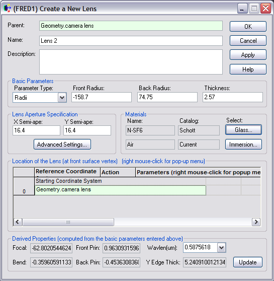
With the camera lens subassembly again highlighted in the Tree, enter the second lens element as shown in Figure 1-6 in much the same manner as Figure 1-4. Select this glass by the same method.

Figure 1-6. Lens 2 for SLR.

Selecting the Apply button will display this lens with its vertex coincident with that of Lens 1. Note from the prescription in Table 1, the thickness between Lens 1 and Lens 2 is 5.14 mm. This spacing is the distance from the 2nd surface of Lens 1 to the first surface of Lens 2. Set this relative spacing by first changing the Starting Coordinate System for Lens 2 to be the 2nd surface of Lens 1. Left-click anywhere inside the green highlighted entry Geometry.camera lens and select the down arrow to expose FRED's Entity Picker dialog. This dialog displays a replica of the Tree as shown below. Select the second surface of Lens 1 and hit the OK button. Geometry.camera lens.Lens 1.Surface 2 should now appear as the Starting Coordinate System of Lens 2. Right-click again and select Append to add shift operation to move Lens 2 into position relative to Lens 1. Type in the 5.14 mm shift as the z-component shift and hit the Apply button to see the lens move to its correct relative position. The clip in Figure 1-7 illustrates this series of steps.

Figure 1-7. Relative referencing of Lens 2 (Video).

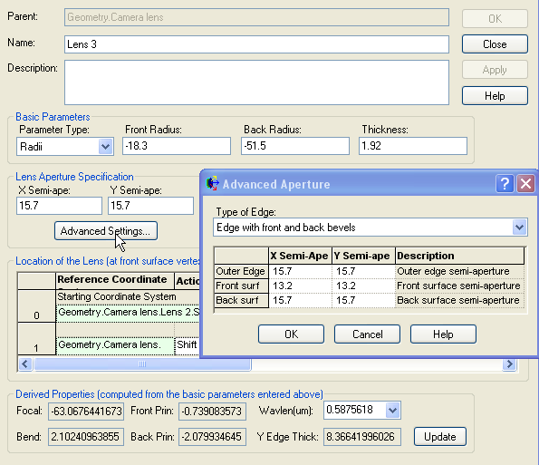
The third and fourth lenses are added to the camera lens subassembly in much the same manner; namely referencing each subsequent lens to the coordinate system of the second surface of its predecessor accompanied by the appropriate air space. In the case of the third lens, specification of different clear apertures for front and back surfaces is handled through the Advanced Settings button under the Lens Aperture Specification using the Edge Type option Edge with front and back bevels as shown in Figure 1-8.

Figure 1-8. Advanced Aperture dialog for Lens 3

Note: For Lens 4 you can replace the Lithosil-Q glass from the Schott catalog with the Fused_Silica material from the Custom catalog.

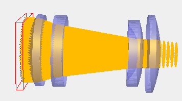
The final camera lens subassembly is shown below in Figure 1-9. Note that as new glasses are added through each Lens dialog, they are automatically added to the Materials folder.

Figure 1-9. Four element camera lens.

Source Primitive Definition

Having completed the camera lens, let us now add a source which yields the stated f/4.3 and determine the plane of best focus. We begin by adding a Source Primitive. This source type can be invoked by four distinct methods:

1.From the Main Menu, Create>Source Primitive>Plane Wave (coherent)

2.Right-click on Optical Sources folder and select option: Create New Source Primitive > Plane Wave (coherent)

3.Create Toolbar button:

Pictured below in Figure 1-10 is the dialog for a Plane Wave (coherent) type Source Primitive in its default state. An elliptical aprture with a 0.5 mm half width is sampled with an 11x11 grid of rays, with all rays are propagating along the z-direction (0,0,1) in the local coordinate system of the source. The source's default coordinate system is the Optical Sources coordinate system which is coincident with the Geometry & Global coordinate systems. The power of the source is 1 Watt. The source's wavelength is 0.5875618 microns, which can be set by the user from the Main Menu Tools>Preferences>Miscellaneous2 under the option "Default Wavelength (mm)."

Figure 1-10. Default Plane Wave (coherent) type Source Primitive dialog.

Next, use the Entity Picker control at the bottom of the source dialog to set the camera lens subassembly as the Starting Coordinate System of the new source.  This action links the source to the camera lens subassembly . Any linear transformations on the camera lens will automatically carry along the source. It is also necessary to shift the source grid to avoid spatial coincidence of the source rays and the camera lens first surface.

Right mouse click (on the "0" of the first row) in the Location/Orientation section of the dialog and choose "Append" from the pop-up menu, which will add a new operation to the source node.  The default operation is a "Shift".  Enter a value of -1 for the Z component of the new Shift operation so that the Location/Orientation portion of the source dialog appears as shown below in Figure 1-11:

Figure 1-11. Shifting the source using the Location/Orientation option.

An approximate x & y semi-aperture of 14.9 mm for the collimated grid is based upon the f-number (f/4.3) and focal length (128.5mm). The number of rays across the grid aperture is somewhat arbitrary at this stage, though this number must be more carefully chosen later on in the Advanced section of this tutorial. An odd number of rays is recommended so as to force a ray to occupy the center of the grid. Therefore, the source grid parameters are as shown below in Figure 1-12:

Figure 1-12. Source parameter configuration

The default wavelength value is acceptable for our application, though you may want to change the Source Draw Color.  When performing a raytrace, the starting source grid and the ray trajectories will be rendered with the chosen color.  This setting is purely a visualization attribute, so feel free to choose your favorite color!

Figure 1-13. Source wavelength attributes

Hit the OK button on the Source Primitive dialog and note that there is now an entry in the Optical Sources folder of the Tree and that the source grid appears in the 3D View as shown in Figure 1-14. When the source (or any other entry in the Tree) is highlighted, that entity is also highlighted in the 3D View.

Figure 1-14. Camera lens with source ray grid.

Note: The source properties in the above dialog and its entry in the Tree represent the definition of how rays will be created prior to a raytrace. No rays actually exist until instructions are given to perform the raytrace.

Basic Raytrace

We are now in position to trace our ray grid through the lens. While there are numerous options for raytracing in FRED, we restrict ourselves at this stage to a basic raytrace initiated by one of three methods:

1.From the Main menu, Raytrace>Trace and Render

2.Keystroke Ctrl+Shft+F7

3.Raytrace Toolbar button

The Trace and Render option creates rays according to the source definition and performs the trace drawing each ray's trajectory. After executing a Trace and Render, you should see the rays traced in FRED's 3D View as shown in Figure 1-15:

Figure 1-15. Trace and Render of source rays through camera lens.

Rays are traced from their creation points with the draw color selected in the previous section through the system to termination. Since all lens surfaces are transmissive, rays exit .camera lens.Lens 4.Surface 2 having no subsequent intersections and are therefore drawn as dashed lines. According to the paradigm by which FRED conducts its raytracing algorithm, all rays shown here are cataloged as being on or associated with .camera lens.Lens 4.Surface 2 (because this was the last surface that the rays hit during the raytrace). When the raytrace completes, FRED prints the Raytrace Summary to the Output Window as in Figure 1-16:

Figure 1-16. Raytrace Summary in Output Window after trace completes.

The Output Window contains the FRED file name, date and time followed by information pertinent to the raytrace. Of particular note here is the last line:

749                    Num rays halted due to no more intersections found (info:1)

The implication here is that all 749 rays have left the system finding no other surface to intersect. Had these rays terminated on an absorbing surface, this message would be absent.

Analysis Tools

Our first order of business with respect to analyses is to confirm the statement in the previous section, i.e., ".....all rays shown here are cataloged as being on or associated with .camera lens.Lens 4.Surface 2." For this job, we use the Ray Summary. This feature is invoked by one of three methods:

1.From the Main Menu, Analyses>Ray Summary

2.Keystroke Shft+F11

3.Analysis Toolbar button

The Ray Summary prints to the Output window a complete listing of number of rays and total incoherent power on each surface along with the surface name. After the raytrace, the Ray Summary produces should produce the output in Figure 1-17 verifying that all rays are currently on camera lens.Lens 4.Surface 2.

Note: The "Total Incoherent Power" column here is not applicable since the source we created is coherent.  Nevertheless, the valuable piece of information provided is that 749 rays are "on" Surface 2 of Lens 4.

Figure 1-17. Ray Summary showing ray count(s), power(s) and surface name(s).

Creation and placement of an image plane has purposely been omitted up to this point. Having set up a source grid which produces the stated f-number of the lens, the final step in completing the SLR camera is to add that image plane. We first must determine its position using a best focus calculation. The Best Geometric Focus feature in FRED is accessed by one of three methods:

1.From the Main Menu, Analyses>Best geometric Focus

2.Keystroke Shft+F9

3.Analysis Toolbar button

The Best Geometric Focus option requires two inputs from the user, 1) the coordinate system in which the best focus position is to be determined, and 2) Ray Selection Criteria which determine which rays are used in the computation. Utilizing relative referencing, we select as the Coordinate System of the Results the entity camera lens.Lens 4.Surface 2 and select as the Ray Selection Criteria "Rays on the specified surface" camera lens.Lens 4.Surface 2 . The movie clip shown in Figure 1-18 illustrates this process:

Figure 1-18. Finding best focus in user-selected coordinate system for specified subset of rays (Video).

FRED prints results of the Best Geometric Focus calculation to the Output Window.  In this case as shown in Figure 1-19 below, the best focus z-position is 56.917 mm from camera lens.Lens 4.Surface 2:

Figure 1-19. Best Geometric Focus output.

In terms of geometry, this tutorial has formally introduced the Subassembly and the Lens as geometric entities. A third entity type, the Element Primitive, will now be introduced.  Element Primitives are a palette of basic objects (plane, sphere, block, pipe, etc.) that can be used as building blocks in your model.  In this example, a Plane type Element Primitive will be used to represent the focal plane.

A Plane type Element Primitive is added to the model by one of the following methods:

1.From the Main Menu, Create > Element Primitive > Plane

2.Create Toolbar button

The new Element Primitive should reside under the camera lens subassembly on your object tree. Therefore, the camera lens subassembly must be highlighted in the Tree before adding the Element Primitive. Initially, note that the Starting Coordinate System of the Element Primitive will be Geometry.camera lens. Use the Entity Picker to select as the Starting Coordinate System as camera lens.Lens 4.Surface 2 consistent with relative referencing and the Best Geometric Focus calculation made above. As recommended practice, the z-shift determined above should be appended to the Position/Orientation operation list of the Element Primitive and will thus also be in the coordinate system of camera lens.Lens 4.Surface 2.  Note, also, that the X and Y semi-apertures of the image plane are set to 2.25 mm.

Figure 1-20. Adding, re-parenting and shifting a Plane type Element Primitive for the Image plane.

When another raytrace is performed, as shown in  Figure 1-21, the rays terminate on the image plane:

Figure 1-21. Raytrace to image plane and Raytrace Summary.

One final element must be added with the intent of performing a Position Spot Diagram at the image plane; an Analysis Surface. The Analysis Surface is used for the following purposes when performing analyses:

•Defines a planar grid of pixels at a specific location in the model.

•Specifies which subset of rays in the model will be included in the analysis.

In the non-sequential raytracing paradigm, the properties of the model's geometry dictate where the rays propagate during the raytrace (as opposed to a sequential paradigm, where the user tells the software where the rays are going).  Consequently, not all rays in the non-sequential model will end on the detector surface(s) at the conclusion of the raytrace.  The second bullet point above indicates that one of the primary functions of the analysis surface is to specify which rays in the model should be included in a given calculation.  Most commonly, the requirement is that "rays on the specified surface" should be included, where the surface specified is the detector surface.

An Analysis Surface can be created by one of the following methods:

1.From the Main Menu, Create>New Analysis Surface

2.Keystroke Ctrl+Alt+N

3.Right-click on Analysis Surface(s) folder and select option <Create New Analysis Surface>

4.Analysis Toolbar button

5.Right-click on the detector surface and select the option, "Auto Create and Attach an Analysis Surface"

In this tutorial we will add an analysis surface using the last method above, since we wish to analyze the ray distribution at the image plane.  Expand the tree node for the "Image" Element Primitive created previously in order to see the "Surface" node underneath it (the "Surface" is a "child" of the "Image" node, in this construction). Right mouse click on the "Surface" node and select, "Auto Create and Attach an Analysis Surface" as shown below in Figure 1-22.  Performing this action will add a new Analysis Surface node to your Analysis Surface(s) folder on the object tree.  The Analysis Surface(s) folder on the object tree can be expanded using the "+" icon to reveal the newly added analysis surface node.

Figure 1-22. Adding an Analysis Surface to the image plane

A Position Spot Diagram of rays at the image plane can now be easily generated. Invoking this feature by one of the following methods:

1.From the Main Menu, Analyses>Position Spot Diagram

2.Keystroke Ctrl+F9

3.Analysis Toolbar button

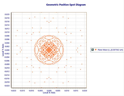
Note that when the Position Spot Diagram is requested, FRED presents the user with a list of available Analysis Surfaces. In general, a FRED model can have an arbitrary number of analysis surfaces defined and the user will need to select the analysis surface intended to be used for the requested calculation.  As only one analysis surface is defined in this tutorial example, simply press OK on the resulting popup dialog in order to perform the Positions Spot Diagram analysis.  Below, Figure 1-23 shows the resulting Positions Spot Diagram calculation for the rays on the image surface.  This analysis reveals the size and distribution of the x,y ray intercept positions on the detector.  Statistical information regarding the size of the "spot diagram" distribution is also printed to the Output Window.

a)          b)

Figure 1-23. a) Spot diagram at best focus position. b) Chart options menu.

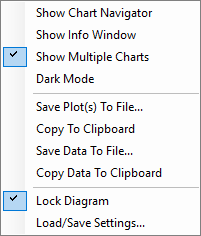
Right-click on the Position Spot Diagram chart to expose a chart attributes menu shown here which allows the Chart Window to be Locked, the Chart Image/Data to be copied to the Clipboard or saved to a file, and access to an advanced "Chart Navigator" menu for more detailed Chart control.

Setup and Perform Paraxial Analysis

FRED can perform a Paraxial Analysis on lens systems as a check on basic performance parameters. However, a Paraxial Analysis implies that the sequence of propagation through the optical system is known.  In order to perform a Paraxial Analysis, a sequential path must be defined using the User-defined Ray Paths feature. The User-defined Ray Paths feature can be accessed by one of the following methods:

1.From the Main Menu, Raytrace>User-defined Raypaths

2.Keystroke Ctrl+Shft+U

3.Raytrace Toolbar button

Open the User-defined Ray Paths dialog and enter the sequential path using the following steps:

1.The default state of the dialog is configured to define a new path.  In the "Definition of currently selected path" portion of the dialog, provide a name for the new path as, "Sequential Path"

2.In Row #0, use the Entity Picker control in the "Surface (or entity)" column to select surface: "Geometry.Camera lens.Lens 1.Surface 1".  The Ray Control setting can be left as "Transmit-Specular", since this is a purely refractive system.

3.In the blank row below, use the Entity Picker control in the "Surface (or entity)" column to select surface: "Geometry.Camera lens.Lens 1.Surface 2".  Again, the Ray Control setting can be left as "Transmit-Specular".

4.Repeat the process above for the remaining optical surfaces:

•"Geometry.Camera lens.Lens 2.Surface 1"

•"Geometry.Camera lens.Lens 2.Surface 2"

•"Geometry.Camera lens.Lens 3.Surface 1"

•"Geometry.Camera lens.Lens 3.Surface 2"

•"Geometry.Camera lens.Lens 4.Surface 1"

•"Geometry.Camera lens.Lens 4.Surface 2"

5.In the last blank row, use the Entity Picker control in the "Surface (or entity)" column to select the image surface, "Geometry.Camera lens.Image.Surface".  Set the Ray Control setting to "Halt", since the rays will be absorbed by the image surface.

6.Hit Apply on the dialog to finish creating the sequential path definition.

The completed Sequential Path definition is shown in the User-defined Ray Paths dialog in Figure 1-24 below.

Figure 1-24. Completed Sequential Path definition.

A Paraxial Analysis can now be carried out on the Sequential Path. Invoke this Analysis feature by one of the following methods:

1.From the Main Menu, Analyses>Paraxial Analysis (first order)

2.Keystroke Shft+F3

3.Analysis Toolbar button

Figure 1-25. Paraxial Analysis dialog based upon sequential path.

Figure 1-25 shows the Paraxial Analysis dialog. The entries in white can be edited to explore various properties of the lens. Buttons on the right provide tabulated output in FRED's Output Window for more detailed analyses. For more information on the Paraxial Analysis, see Help.

Note: When lens prescriptions are imported as will be done in the next section, FRED learns both a DefaultSequential and ReverseSequential path automatically.

Once this tutorial is completed, save the file for use elsewhere. We will come back to this FRED file and perform some addition analyses.